Spatial Data - Displaying time series, spatial and space-time data with R
Table of Contents
Proportional symbol mapping
Interactive Graphics
mapView
GeoJSON
rgl
Choropleth maps
Interactive Graphics
Raster maps
Interactive Graphics
Vector fields
Physical maps
Reference maps
Code
Choropleth maps
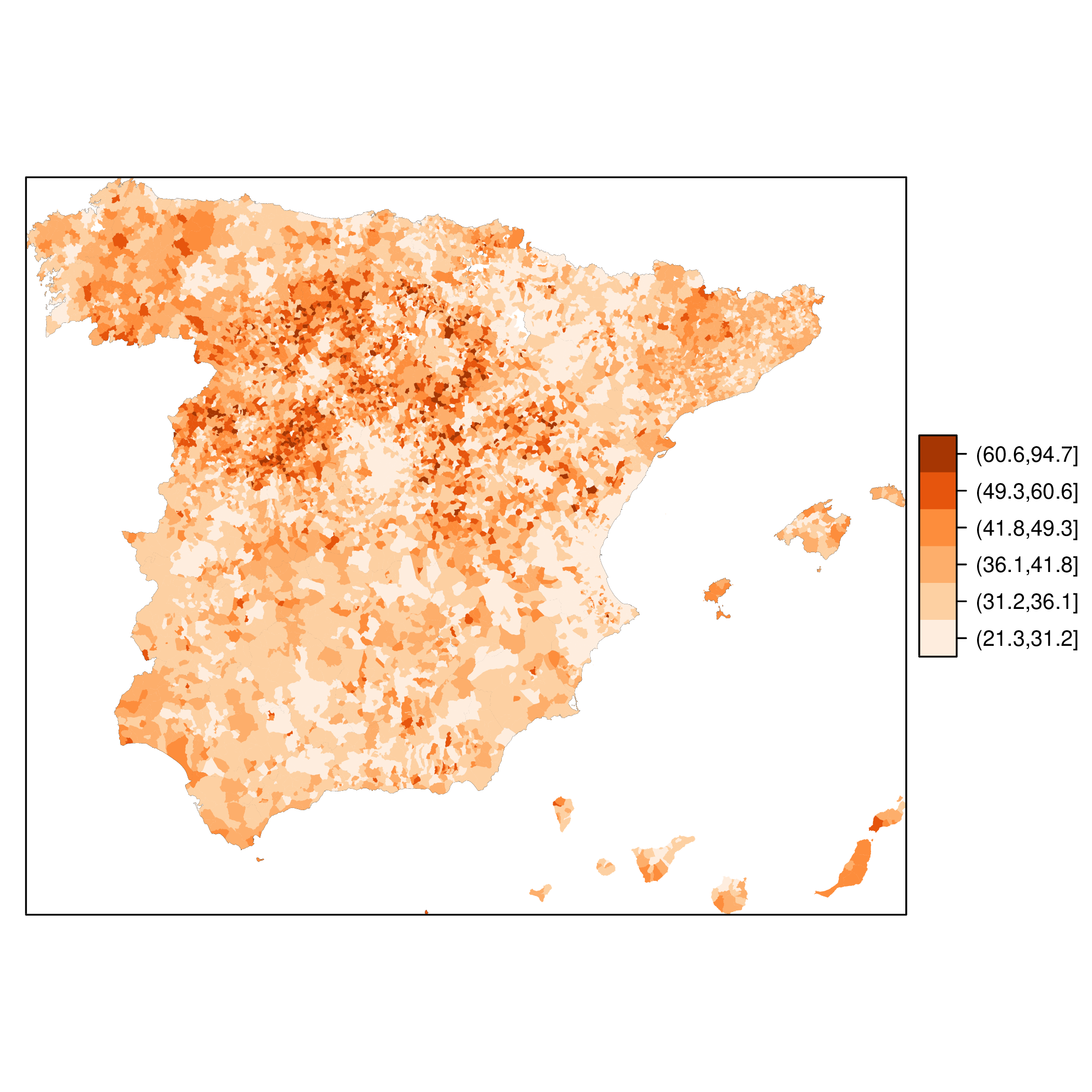
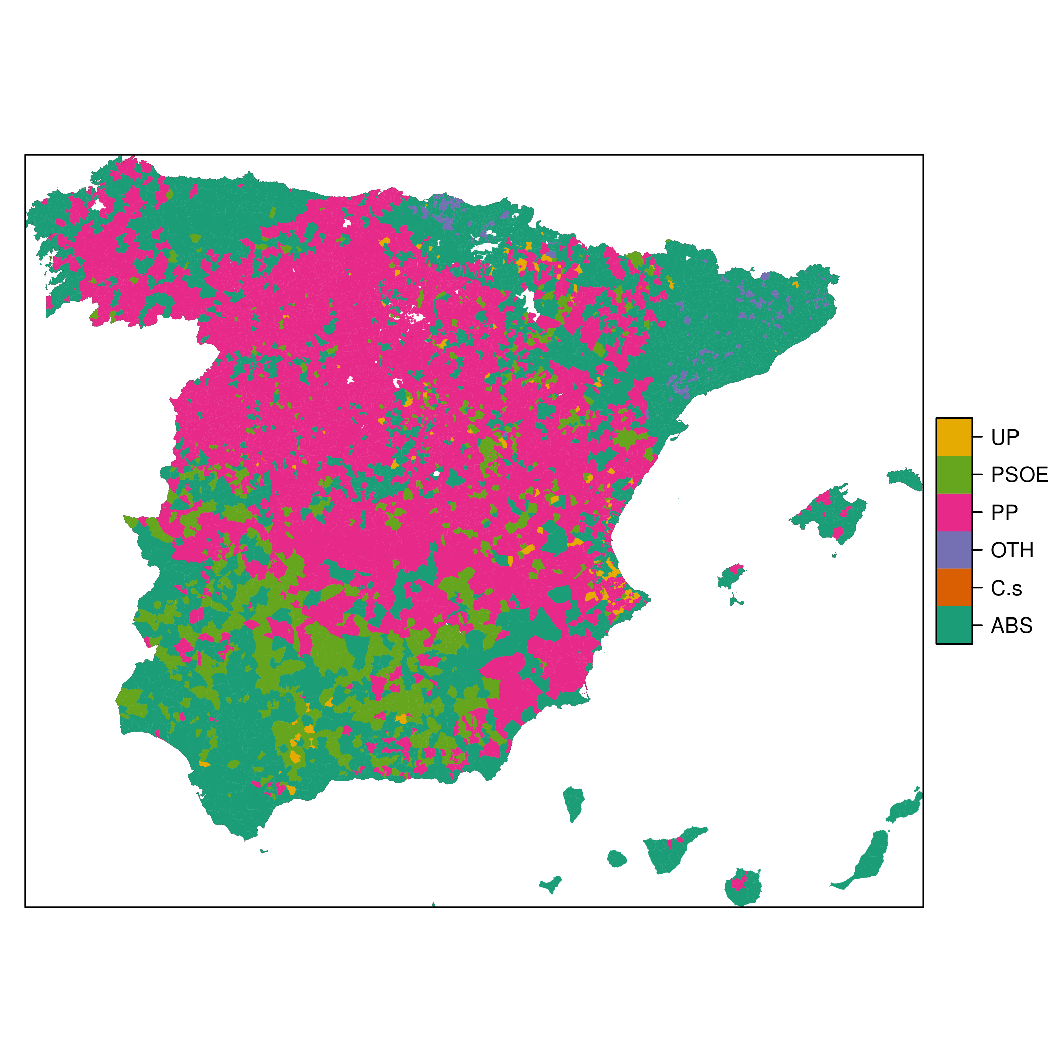
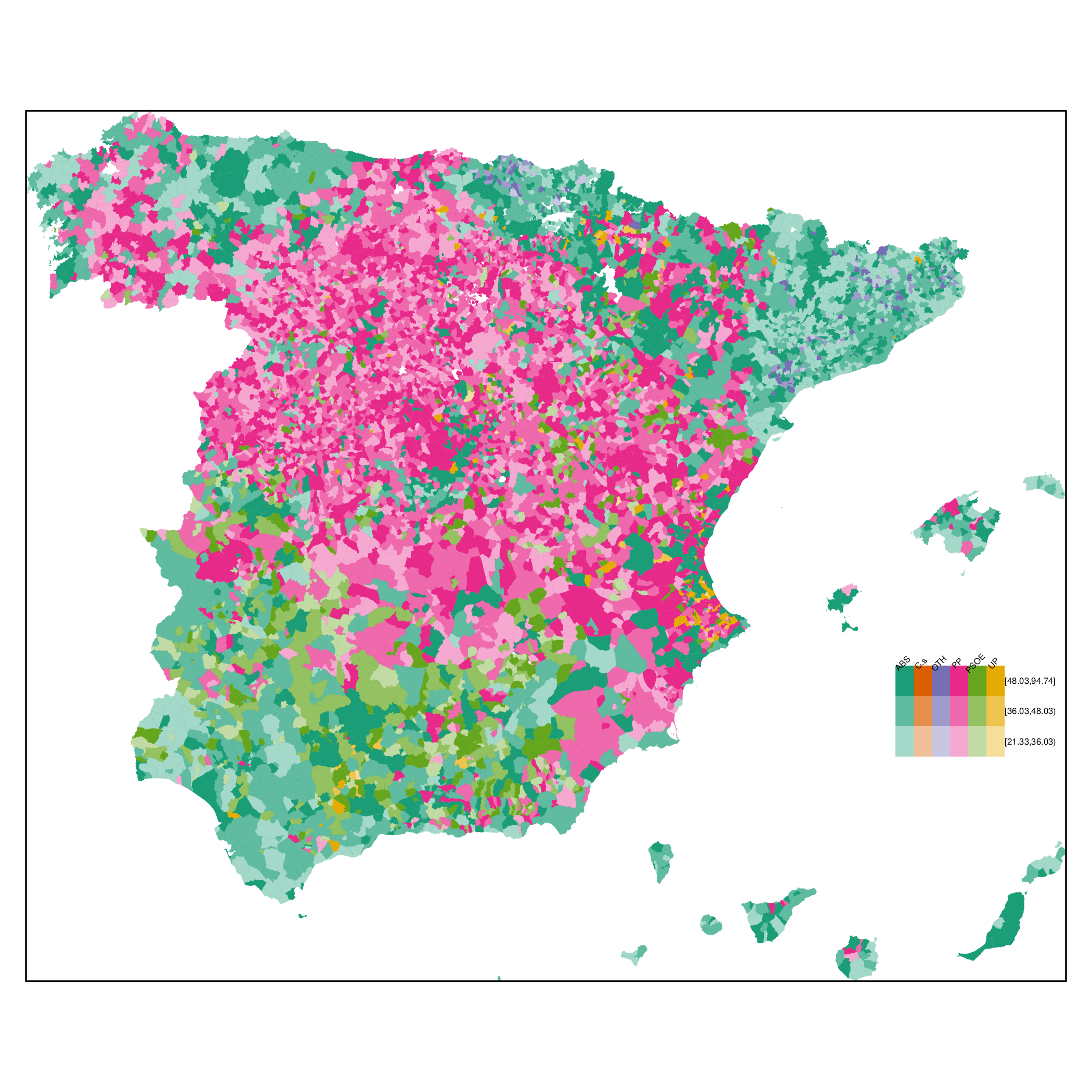
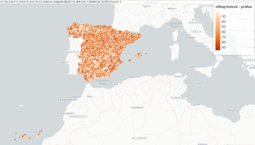
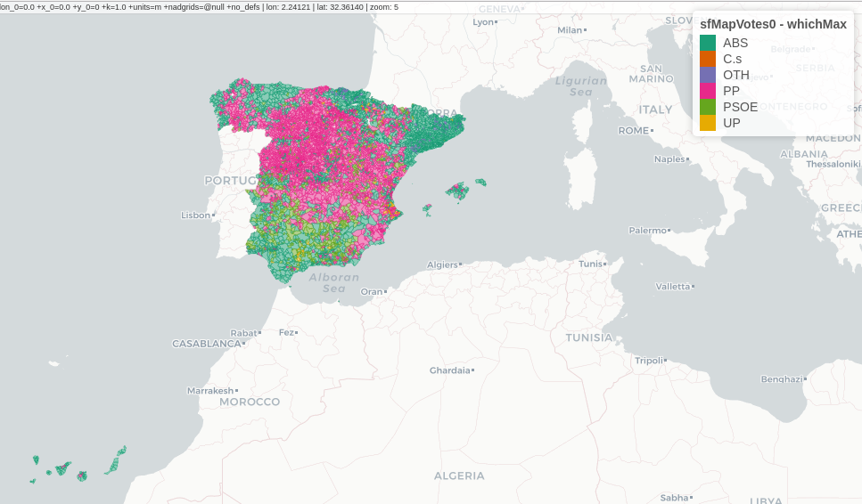
##################################################################
## Initial configuration
##################################################################
## Clone or download the repository and set the working directory
## with setwd to the folder where the repository is located.

library(lattice)
library(ggplot2)
## latticeExtra must be loaded after ggplot2 to prevent masking of its
## `layer` function.
library(latticeExtra)

source('configLattice.R')
##################################################################

##################################################################
## Read data
##################################################################

## sp approach
library(sp)
library(rgdal)

spMapVotes <- readOGR("data/spMapVotes.shp",
                      p4s = "+proj=utm +zone=30 +ellps=GRS80 +units=m +no_defs")

## sf approach
library(sf)

sfMapVotes <- st_read("data/spMapVotes.shp")
st_crs(sfMapVotes) <- 25830

##################################################################
## Province Boundaries
##################################################################

## sp
provinces <- readOGR("data/spain_provinces.shp",
                     p4s = "+proj=utm +zone=30 +ellps=GRS80 +units=m +no_defs")

provinceLines <- list("sp.polygons", provinces, lwd = 0.1)

## sf
sfProvs <- st_read("data/spain_provinces.shp")
st_crs(sfProvs) <- 25830

##################################################################
## Quantitative variable
##################################################################

library(RColorBrewer)

## Number of intervals (colors)
N <- 6
## Sequential palette
quantPal <- brewer.pal(n = N, "Oranges")

## Number of cuts
ucN <- 1000
## Palette created with interpolation
ucQuantPal <- colorRampPalette(quantPal)(ucN)

## The polygons boundaries are not displayed thanks to col = 'transparent'
spplot(spMapVotes["pcMax"],
       col.regions = ucQuantPal,
       cuts = ucN,
       ## Do not draw municipality boundaries
       col = 'transparent',
       ## Overlay province boundaries
       sp.layout = provinceLines)

##################################################################
## Data classification
##################################################################

ggplot(as.data.frame(spMapVotes),
       aes(pcMax,
           fill = whichMax,
           colour = whichMax)) +
    geom_density(alpha = 0.1) +
    theme_bw()

library(classInt)

## Compute intervals with the same number of elements
intQuant <- classIntervals(spMapVotes$pcMax,
                           n = N, style = "quantile")
## Compute intervals with the natural breaks algorithm
intFisher <- classIntervals(spMapVotes$pcMax,
                            n = N, style = "fisher")

plot(intQuant, pal = quantPal, main = "")

plot(intFisher, pal = quantPal, main = "")

## spplot solution

## Add a new categorical variable with cut, using the computed breaks
spMapVotes$pcMaxInt <- cut(spMapVotes$pcMax,
                            breaks = intFisher$brks)

spplot(spMapVotes["pcMaxInt"],
       col = 'transparent',
       col.regions = quantPal,
       sp.layout = provinceLines)

## sf and geom_sf
sfMapVotes$pcMaxInt <- cut(sfMapVotes$pcMax,
                           breaks = intFisher$brks)

ggplot(sfMapVotes) +
    ## Display the pcMaxInt variable...
    geom_sf(aes(fill = pcMaxInt),
            ## without drawing municipality boundaries
            color = "transparent") +
    scale_fill_brewer(palette = "Oranges") +
    ## And overlay provinces boundaries
    geom_sf(data = sfProvs,
            fill = 'transparent',
            ## but do not include them in the legend
            show.legend = FALSE) +
    theme_bw()

##################################################################
## Qualitative variable
##################################################################

classes <- levels(factor(spMapVotes$whichMax))
nClasses <- length(classes)

qualPal <- brewer.pal(nClasses, "Dark2")

## spplot solution
spplot(spMapVotes["whichMax"],
       col.regions = qualPal,
       col = 'transparent',
       sp.layout = provinceLines)

## geom_sf solution
ggplot(sfMapVotes) +
    geom_sf(aes(fill = whichMax),
            color = "transparent") +
    scale_fill_brewer(palette = 'Dark2') +
    geom_sf(data = sfProvs,
            fill = 'transparent',
            show.legend = FALSE) +
    theme_bw()

##################################################################
## Small multiples
##################################################################

## spplot version
spplot(spMapVotes, "pcMaxInt",
       ## Formula to define the faceting: a panel for each level of
       ## whichMax
       formula = pcMaxInt ~ xlabelpoint + ylabelpoint | whichMax,
       col.regions = quantPal,
       col = 'transparent',
       sp.layout = provinceLines)

## ggplot2 version
ggplot(sfMapVotes) +
    geom_sf(aes(fill = pcMaxInt),
            color = "transparent") +
    ## Define the faceting using two rows
    facet_wrap(~whichMax, nrow = 2) +
    scale_fill_brewer(palette = "Oranges") +
    geom_sf(data = sfProvs,
            fill = 'transparent',
            size = 0.1,
            show.legend = FALSE) +
    theme_bw()

##################################################################
## Bivariate map
##################################################################

## Number of intervals.
N <- 3
## Loop to create a bidimensional palette
multiPal <- sapply(1:nClasses, function(i)
{
    colorAlpha <- adjustcolor(qualPal[i], alpha = 0.4)
    colorRampPalette(c(qualPal[i], colorAlpha), alpha = TRUE)(N)
})

## Define the intervals
intFisher <- classIntervals(spMapVotes$pcMax,
                            n = N, style = "fisher")
## ... and create a categorical variable with them
spMapVotes$pcMaxInt <- cut(spMapVotes$pcMax,
                            breaks = intFisher$brks)

pList <- lapply(1:nClasses, function(i){
    ## Only those polygons corresponding to a level are selected
    mapClass <- subset(spMapVotes,
                       whichMax == classes[i])
    ## Palette
    pal <- multiPal[, i]
    ## Produce the graphic
    pClass <- spplot(mapClass, "pcMaxInt",
                     col.regions = pal,
                     col = 'transparent',
                     colorkey = FALSE)
})
names(pList) <- classes
p <- Reduce('+', pList)

op <- options(digits = 4)
tabFisher <- print(intFisher)
intervals <- names(tabFisher)
options(op)

library(grid)

legend <- layer(
{
    ## Position of the legend
    x0 <- 1000000
    y0 <- 4200000
    ## Width of the legend
    w <- 120000
    ## Height of the legend
    h <- 100000
    ## Colors
    grid.raster(multiPal, interpolate = FALSE,
                      x = unit(x0, "native"),
                      y = unit(y0, "native"),
                width = unit(w, "native"),
                height = unit(h, "native"))
    ## x-axis (qualitative variable)
    grid.text(classes,
              x = unit(seq(x0 - w * (nClasses -1)/(2*nClasses),
                           x0 + w * (nClasses -1)/(2*nClasses),
                           length = nClasses),
                       "native"),
              y = unit(y0 + h/2, "native"),
              just = "bottom",
              rot = 10,
              gp = gpar(fontsize = 4))
    ## y-axis (quantitative variable)
    Ni <- length(intervals)
    grid.text(intervals,
              x = unit(x0 + w/2, "native"),
              y = unit(seq(y0 - h * (Ni -1)/(2*Ni),
                           y0 + h * (Ni -1)/(2*Ni),
                           length = Ni),
                       "native"),
              just = "left",
              gp = gpar(fontsize = 6))
})

## Main plot
p + legend

##################################################################
## Interactive Graphics
##################################################################

library(mapview)

sfMapVotes0 <- st_read("data/spMapVotes0.shp")
st_crs(sfMapVotes0) <- 25830

## Quantitative variable, pcMax
mapView(sfMapVotes0,
        zcol = "pcMax", ## Choose the variable to display
        legend = TRUE,
        col.regions = quantPal)

## Qualitative variable, whichMax
mapView(sfMapVotes0,
        zcol = "whichMax",
        legend = TRUE,
        col.regions = qualPal)
Raster maps
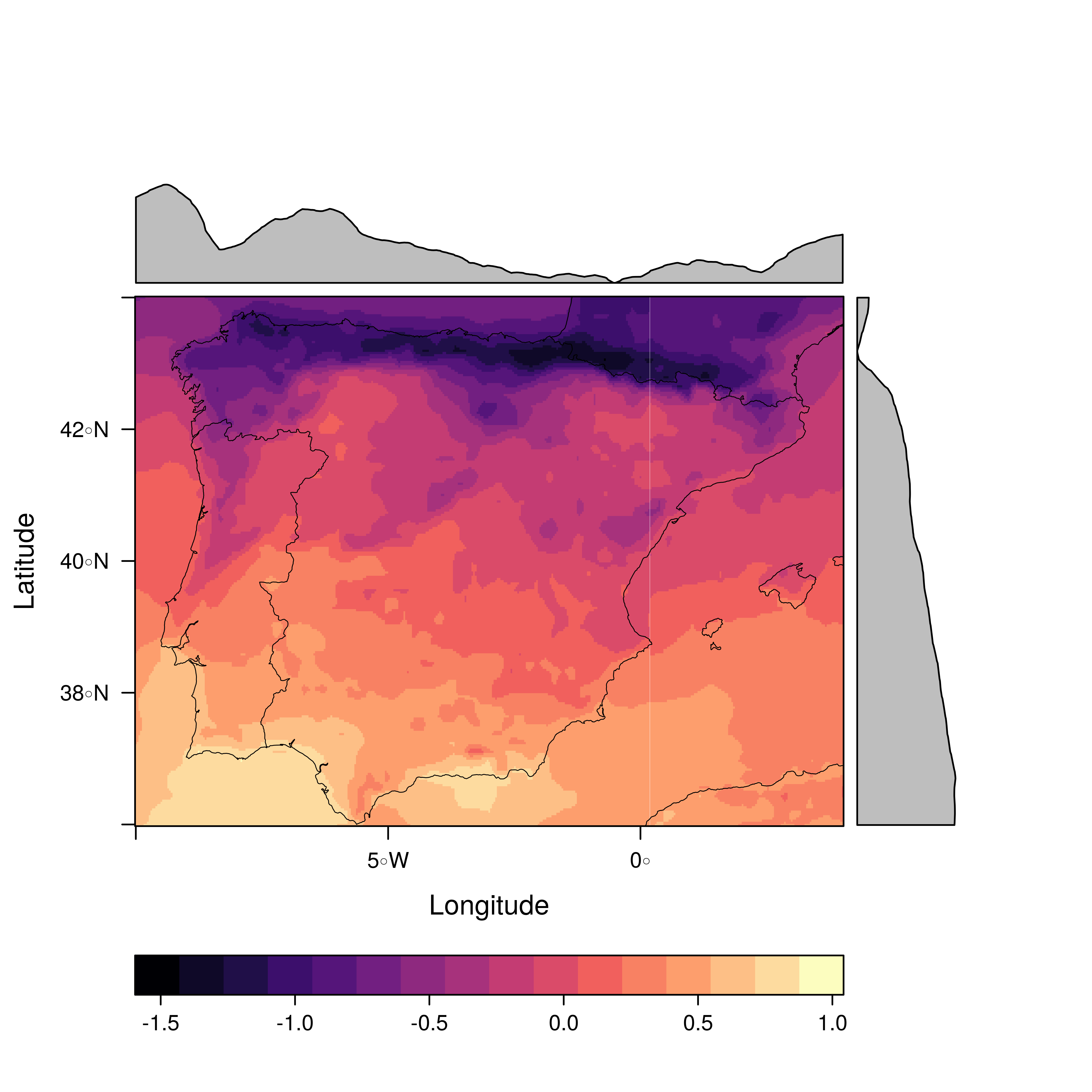
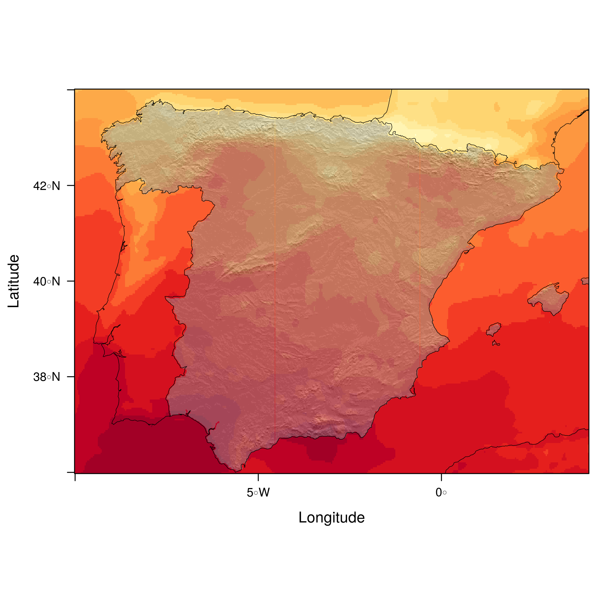
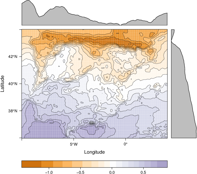
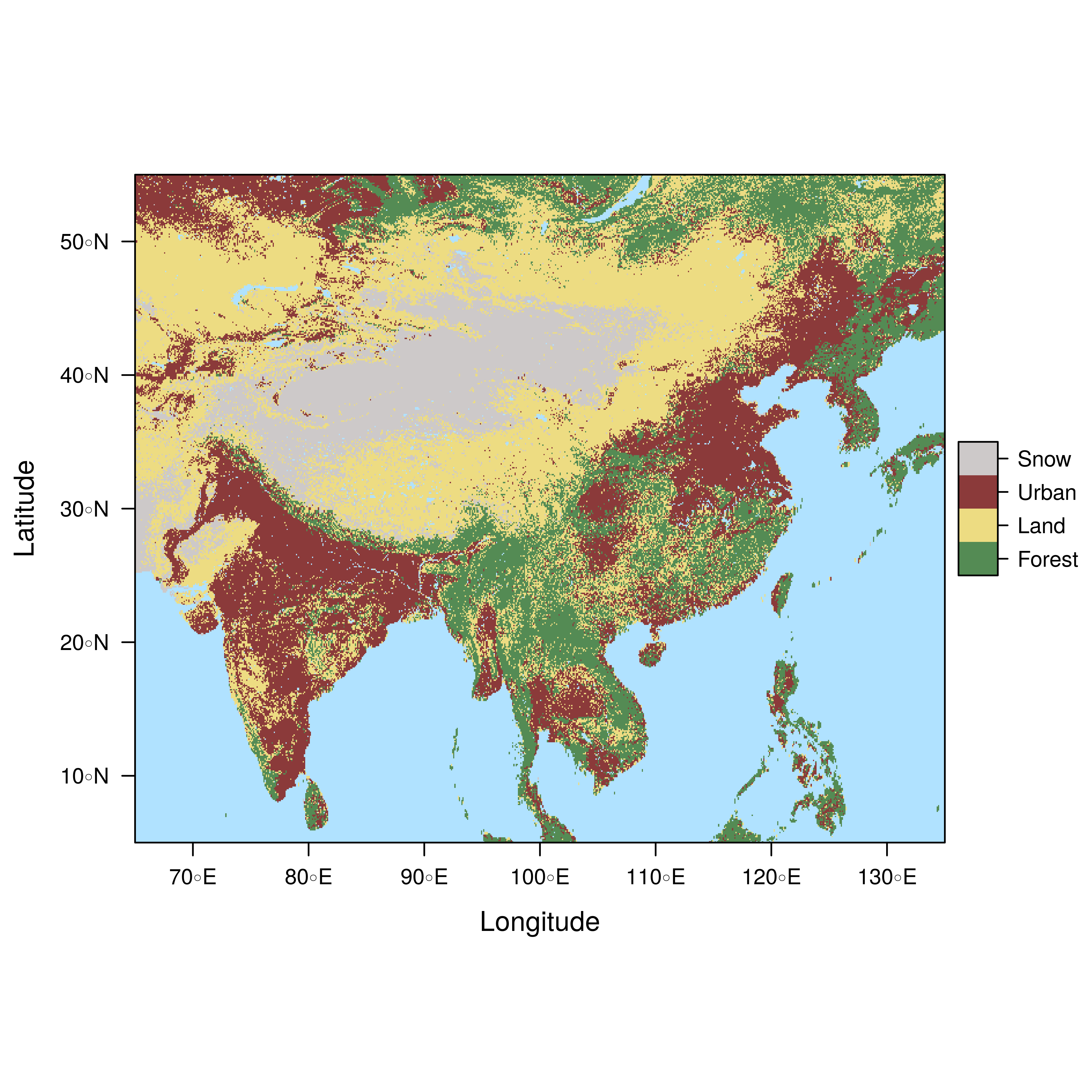
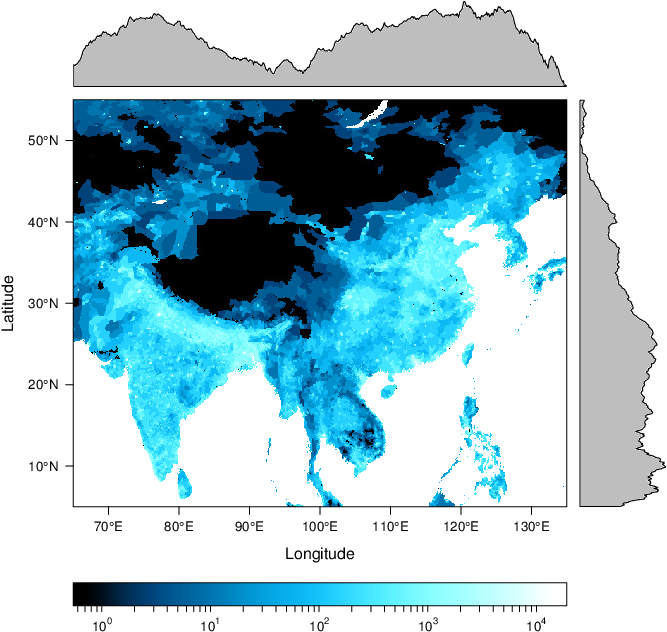
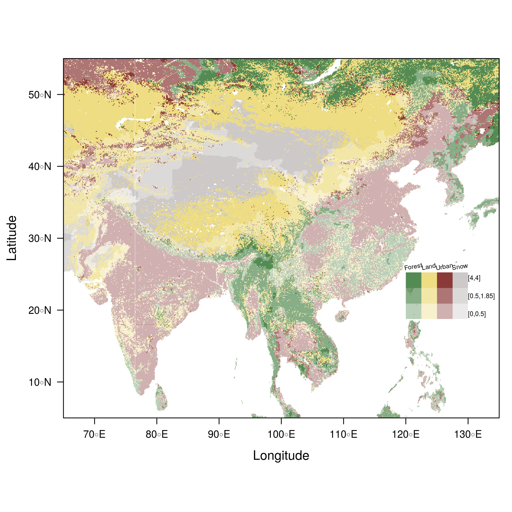
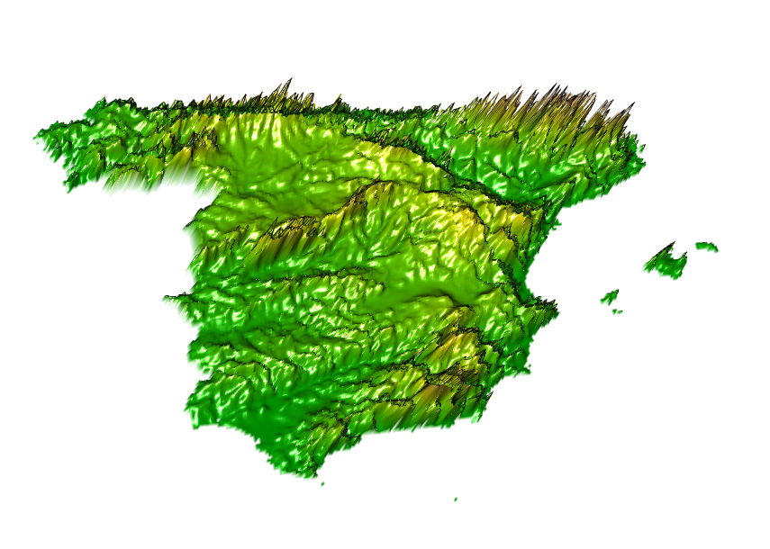
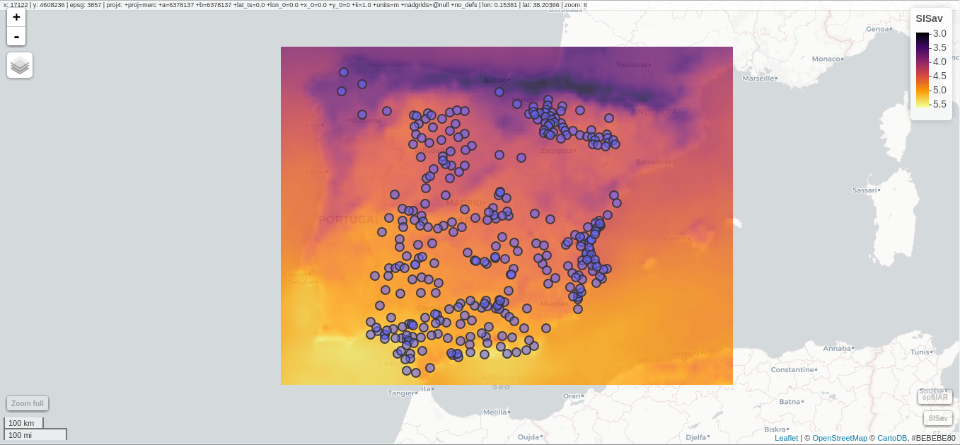
##################################################################
## Initial configuration
##################################################################
## Clone or download the repository and set the working directory
## with setwd to the folder where the repository is located.

##################################################################
## Quantitative data
##################################################################

library(raster)
library(rasterVis)

SISav <- raster('data/SISav')

levelplot(SISav)

library(maps)
library(mapdata)
library(maptools)
## Extent of the Raster object
ext <- as.vector(extent(SISav))
## Retrieve the boundaries restricted to this extent
boundaries <- map('worldHires',
                  xlim = ext[1:2], ylim = ext[3:4],
                  plot = FALSE)
## Convert the result to a SpatialLines object with the projection of
## the Raster object
boundaries <- map2SpatialLines(boundaries,
                               proj4string = CRS(projection(SISav)))

## Display the Raster object ...
levelplot(SISav) +
    ## ... and overlay the SpatialLines object
    layer(sp.lines(boundaries,
                   lwd = 0.5))

##################################################################
## Hill shading
##################################################################

old <- setwd(tempdir())
download.file('http://biogeo.ucdavis.edu/data/diva/msk_alt/ESP_msk_alt.zip', 'ESP_msk_alt.zip')
unzip('ESP_msk_alt.zip', exdir = '.')

DEM <- raster('ESP_msk_alt')

slope <- terrain(DEM, 'slope')
aspect <- terrain(DEM, 'aspect')
hs <- hillShade(slope = slope, aspect = aspect,
                angle = 60, direction = 45)

setwd(old)

## hillShade theme: gray colors and semitransparency
hsTheme <- GrTheme(regions = list(alpha = 0.5))

levelplot(SISav,
          par.settings = YlOrRdTheme,
          margin = FALSE, colorkey = FALSE) +
    ## Overlay the hill shade raster
    levelplot(hs, par.settings = hsTheme, maxpixels = 1e6) +
    ## and the countries boundaries
    layer(sp.lines(boundaries, lwd = 0.5))

##################################################################
## Diverging palettes
##################################################################

meanRad <- cellStats(SISav, 'mean')
SISav <- SISav - meanRad

xyplot(layer ~ y, data = SISav,
       groups = cut(x, 5),
       par.settings = rasterTheme(symbol = plinrain(n = 5,
                                                    end = 200)),
       xlab = 'Latitude', ylab = 'Solar radiation (scaled)',
       auto.key = list(space = 'right',
                       title = 'Longitude',
                       cex.title = 1.3))

divPal <- brewer.pal(n = 9, 'PuOr')
divPal[5] <- "#FFFFFF"

showPal <- function(pal)
{
    N <- length(pal)
    image(1:N, 1, as.matrix(1:N), col = pal,
          xlab = '', ylab = '',
          xaxt = "n", yaxt = "n",
          bty = "n")
}

showPal(divPal)

divTheme <- rasterTheme(region = divPal)

levelplot(SISav, contour = TRUE, par.settings = divTheme)

rng <- range(SISav[])
## Number of desired intervals
nInt <- 15
## Increment corresponding to the range and nInt
inc0 <- diff(rng)/nInt
## Number of intervals from the negative extreme to zero
n0 <- floor(abs(rng[1])/inc0)
## Update the increment adding 1/2 to position zero in the center of an interval
inc <- abs(rng[1])/(n0 + 1/2)
## Number of intervals from zero to the positive extreme
n1 <- ceiling((rng[2]/inc - 1/2) + 1)
## Collection of breaks
breaks <- seq(rng[1], by = inc, length= n0 + 1 + n1)

## Midpoints computed with the median of each interval
idx <- findInterval(SISav[], breaks, rightmost.closed = TRUE)
mids <- tapply(SISav[], idx, median)
## Maximum of the absolute value both limits
mx <- max(abs(breaks))

break2pal <- function(x, mx, pal){
    ## x = mx gives y = 1
    ## x = 0 gives y = 0.5
    y <- 1/2*(x/mx + 1)
    rgb(pal(y), maxColorValue = 255)
}

## Interpolating function that maps colors with [0, 1]
## rgb(divRamp(0.5), maxColorValue=255) gives "#FFFFFF" (white)
divRamp <- colorRamp(divPal)
## Diverging palette where white is associated with the interval
## containing the zero
pal <- break2pal(mids, mx, divRamp)
showPal(pal)

levelplot(SISav,
          par.settings = rasterTheme(region = pal),
          at = breaks, contour = TRUE)

divTheme <- rasterTheme(regions = list(col = pal))

levelplot(SISav,
          par.settings = divTheme,
          at = breaks,
          contour = TRUE)

library(classInt)

cl <- classIntervals(SISav[], style = 'kmeans')
breaks <- cl$brks

## Repeat the procedure previously exposed, using the 'breaks' vector
## computed with classIntervals
idx <- findInterval(SISav[], breaks, rightmost.closed = TRUE)
mids <- tapply(SISav[], idx, median)

mx <- max(abs(breaks))
pal <- break2pal(mids, mx, divRamp)

## Modify the vector of colors in the 'divTheme' object
divTheme$regions$col <- pal

levelplot(SISav,
          par.settings = divTheme,
          at = breaks,
          contour = TRUE)

##################################################################
## Categorical data
##################################################################

## China and India
ext <- extent(65, 135, 5, 55)

pop <- raster('data/875430rgb-167772161.0.FLOAT.TIFF')
pop <- crop(pop, ext)
pop[pop==99999] <- NA

landClass <- raster('data/241243rgb-167772161.0.TIFF')
landClass <- crop(landClass, ext)

landClass[landClass %in% c(0, 254)] <- NA
## Only four groups are needed:
## Forests: 1:5
## Shrublands, etc: 6:11
## Agricultural/Urban: 12:14
## Snow: 15:16
landClass <- cut(landClass, c(0, 5, 11, 14, 16))
## Add a Raster Attribute Table and define the raster as categorical data
landClass <- ratify(landClass)
## Configure the RAT: first create a RAT data.frame using the
## levels method; second, set the values for each class (to be
## used by levelplot); third, assign this RAT to the raster
## using again levels
rat <- levels(landClass)[[1]]
rat$classes <- c('Forest', 'Land', 'Urban', 'Snow')
levels(landClass) <- rat

qualPal <- c('palegreen4', # Forest
         'lightgoldenrod', # Land
         'indianred4', # Urban
         'snow3')      # Snow

qualTheme <- rasterTheme(region = qualPal,
                        panel.background = list(col = 'lightskyblue1')
                        )

levelplot(landClass, maxpixels = 3.5e5,
          par.settings = qualTheme)

pPop <- levelplot(pop, zscaleLog = 10,
                  par.settings = BTCTheme,
                  maxpixels = 3.5e5)
pPop

## Join the RasterLayer objects to create a RasterStack object.
s <- stack(pop, landClass)
names(s) <- c('pop', 'landClass')

densityplot(~log10(pop), ## Represent the population
            groups = landClass, ## grouping by land classes
            data = s,
            ## Do not plot points below the curves
            plot.points = FALSE)

##################################################################
## Bivariate legend
##################################################################

classes <- rat$classes
nClasses <- length(classes)

logPopAt <- c(0, 0.5, 1.85, 4)

nIntervals <- length(logPopAt) - 1

multiPal <- sapply(1:nClasses, function(i)
{
    colorAlpha <- adjustcolor(qualPal[i], alpha = 0.4)
    colorRampPalette(c(qualPal[i],
                       colorAlpha),
                     alpha = TRUE)(nIntervals)
})

pList <- lapply(1:nClasses, function(i){
    landSub <- landClass
    ## Those cells from a different land class are set to NA...
    landSub[!(landClass==i)] <- NA
    ## ... and the resulting raster masks the population raster
    popSub <- mask(pop, landSub)
    ## Palette
    pal <- multiPal[, i]

    pClass <- levelplot(log10(popSub),
                        at = logPopAt,
                        maxpixels = 3.5e5,
                        col.regions = pal,
                        colorkey = FALSE,
                        margin = FALSE)
})

p <- Reduce('+', pList)

library(grid)

legend <- layer(
{
    ## Center of the legend (rectangle)
    x0 <- 125
    y0 <- 22
    ## Width and height of the legend
    w <- 10
    h <- w / nClasses * nIntervals
    ## Legend
    grid.raster(multiPal, interpolate = FALSE,
                      x = unit(x0, "native"),
                      y = unit(y0, "native"),
                width = unit(w, "native"))
    ## Axes of the legend
    ## x-axis (qualitative variable)
    grid.text(classes,
              x = unit(seq(x0 - w * (nClasses -1)/(2*nClasses),
                           x0 + w * (nClasses -1)/(2*nClasses),
                           length = nClasses),
                       "native"),
              y = unit(y0 + h/2, "native"),
              just = "bottom",
              rot = 10,
              gp = gpar(fontsize = 6))
    ## y-axis (quantitative variable)
    yLabs <- paste0("[",
                    paste(logPopAt[-nIntervals],
                          logPopAt[-1], sep = ","),
                    "]")
    grid.text(yLabs,
              x = unit(x0 + w/2, "native"),
              y = unit(seq(y0 - h * (nIntervals -1)/(2*nIntervals),
                           y0 + h * (nIntervals -1)/(2*nIntervals),
                           length = nIntervals),
                       "native"),
              just = "left",
              gp = gpar(fontsize = 6))

})

p + legend

##################################################################
## 3D visualization
##################################################################

plot3D(DEM, maxpixels = 5e4)

## Dimensions of the window in pixels
par3d(viewport = c(0, 30, ## Coordinates of the lower left corner
                   250, 250)) ## Width and height

writeWebGL(filename = 'docs/images/rgl/DEM.html',
           width = 800)

##################################################################
## mapview
##################################################################

library(mapview)

mvSIS <- mapview(SISav, legend = TRUE)

SIAR <- read.csv("data/SIAR.csv")

spSIAR <- SpatialPointsDataFrame(coords = SIAR[, c("lon", "lat")],
                                 data = SIAR,
                                 proj4str = CRS(projection(SISav)))

mvSIAR <- mapview(spSIAR,
                  label = spSIAR$Estacion)

mvSIS + mvSIAR
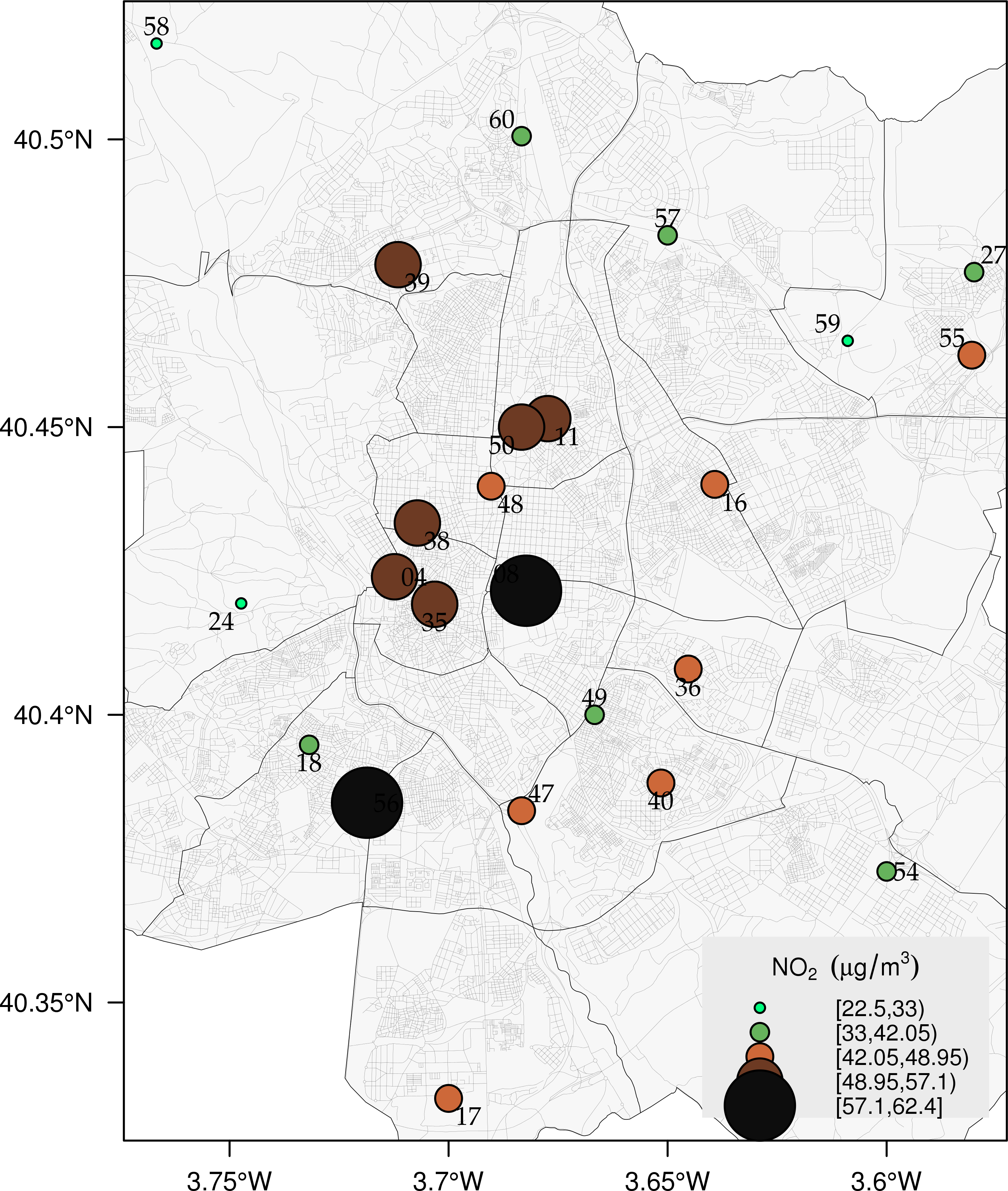
Proportional symbol mapping
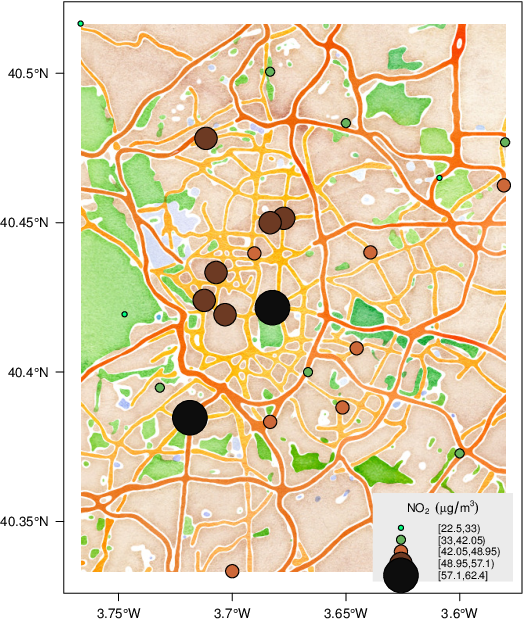
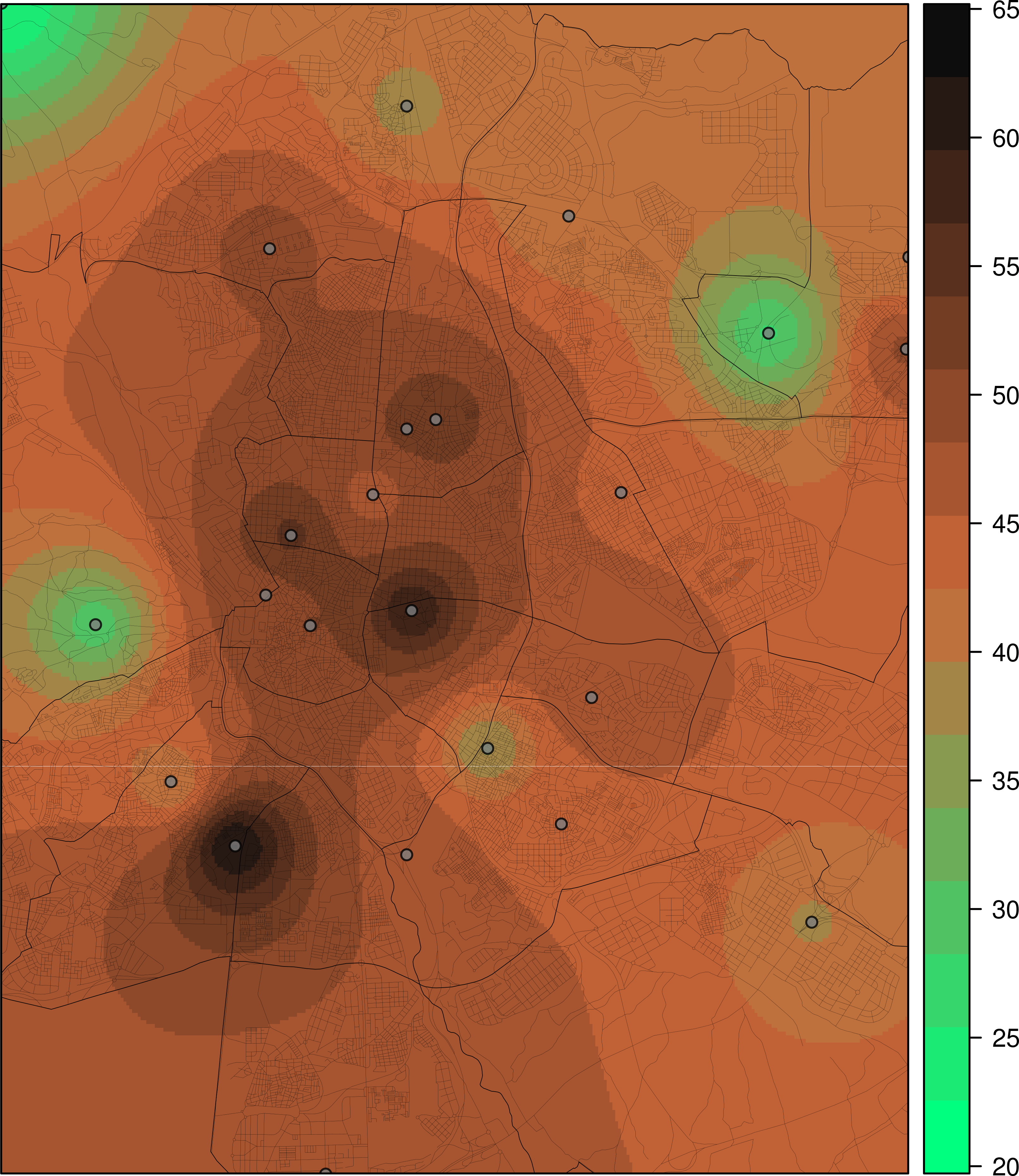
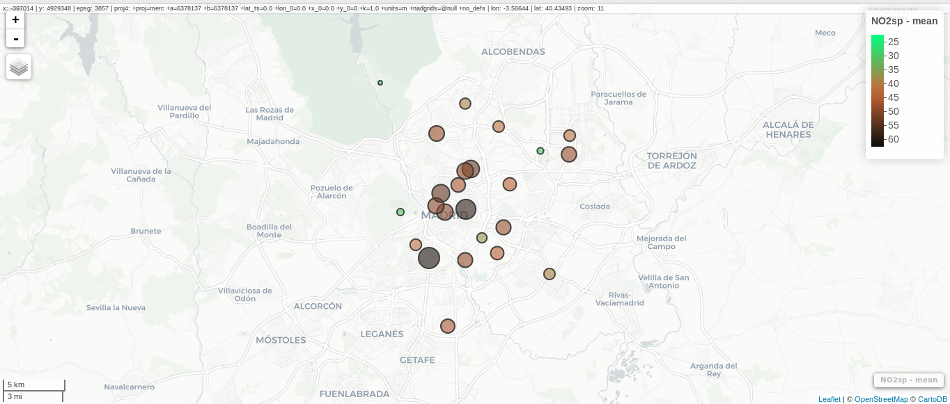
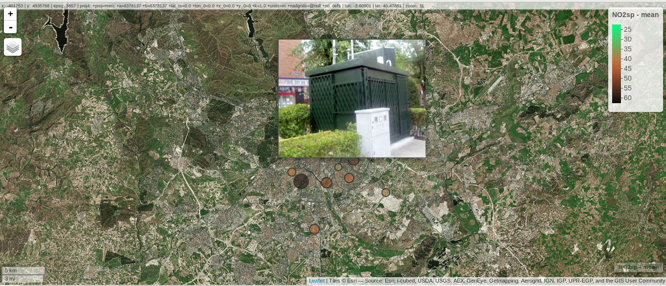
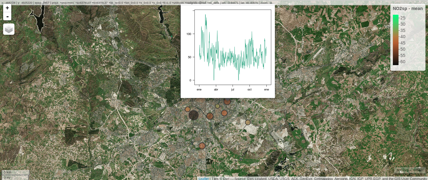
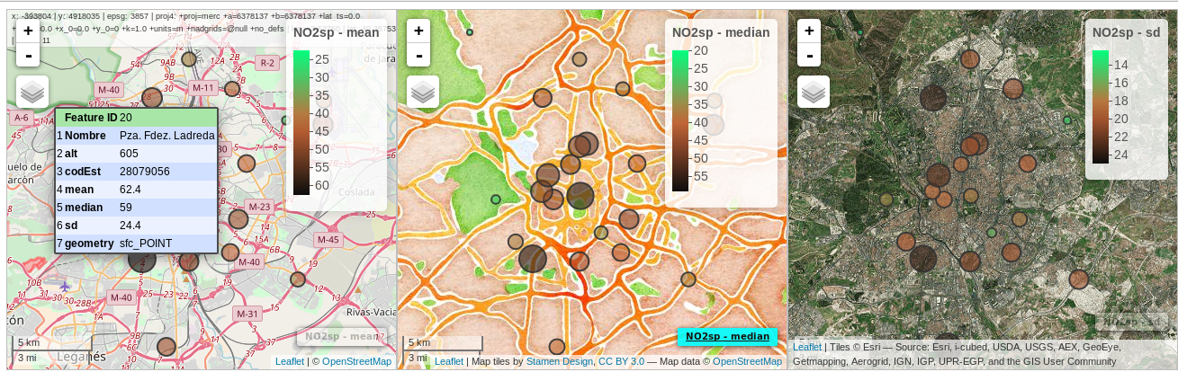
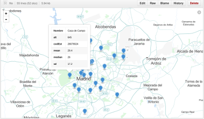
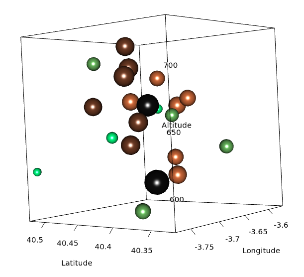
##################################################################
## Initial configuration
##################################################################
## Clone or download the repository and set the working directory
## with setwd to the folder where the repository is located.

library(lattice)
library(ggplot2)
## latticeExtra must be loaded after ggplot2 to prevent masking of its
## `layer` function.
library(latticeExtra)

source('configLattice.R')
##################################################################

##################################################################
## Proportional symbol with spplot
##################################################################

library(sp)
library(rgdal)

NO2sp <- readOGR(dsn = 'data/', layer = 'NO2sp')

airPal <- colorRampPalette(c('springgreen1', 'sienna3', 'gray5'))(5)

spplot(NO2sp["mean"],
       col.regions = airPal, ## Palette
       cex = sqrt(1:5), ## Size of circles
       edge.col = 'black', ## Color of border
       scales = list(draw = TRUE), ## Draw scales
       key.space = 'right') ## Put legend on the right

##################################################################
## Proportional symbol with ggplot
##################################################################

library(sf)

NO2sf <- st_read(dsn = 'data', layer = 'NO2sp')
## Create a categorical variable
NO2sf$Mean <- cut(NO2sf$mean, 5)

ggplot(data = NO2sf) +
    geom_sf(aes(size = Mean, fill = Mean),
            pch = 21, col = 'black') +
    scale_fill_manual(values = airPal) +
    theme_bw()

##################################################################
## Optimal classification and sizes to improve discrimination
##################################################################

library(classInt)
## The number of classes is chosen between the Sturges and the
## Scott rules.
nClasses <- 5
intervals <- classIntervals(NO2sp$mean, n = nClasses, style = 'fisher')
## Number of classes is not always the same as the proposed number
nClasses <- length(intervals$brks) - 1

op <- options(digits = 4)
tab <- print(intervals)
options(op)

## Complete Dent set of circle radii (mm)
dent <- c(0.64, 1.14, 1.65, 2.79, 4.32, 6.22, 9.65, 12.95, 15.11)
## Subset for our dataset
dentAQ <- dent[seq_len(nClasses)]
## Link Size and Class: findCols returns the class number of each
## point; cex is the vector of sizes for each data point
idx <- findCols(intervals)
cexNO2 <- dentAQ[idx]

## spplot version
NO2sp$classNO2 <- factor(names(tab)[idx])

## Definition of an improved key with title and background
NO2key <- list(x = 0.99, y = 0.01, corner = c(1, 0),
               title = expression(NO[2]~~(paste(mu, plain(g))/m^3)),
               cex.title = 0.8, cex = 1,
               background = 'gray92')

pNO2 <- spplot(NO2sp["classNO2"],
               col.regions = airPal,
               cex = dentAQ * 0.8,
               edge.col = 'black',
               scales = list(draw = TRUE),
               key.space = NO2key)
pNO2

## ggplot2 version
NO2sf$classNO2 <- factor(names(tab)[idx])

ggplot(data = NO2sf) +
    geom_sf(aes(size = classNO2, fill = classNO2),
            pch = 21, col = 'black') +
    scale_fill_manual(values = airPal) +
    scale_size_manual(values = dentAQ * 2)  +
    xlab("") + ylab("") + theme_bw()

##################################################################
## Spatial context with underlying layers and labels
##################################################################

##################################################################
## Static image
##################################################################

## Bounding box of data
madridBox <- bbox(NO2sp)
## Extend the limits to get a slightly larger map
madridBox <- t(apply(madridBox, 1,
                   extendrange, f = 0.05))

library(ggmap)

madridGG <- get_map(c(madridBox),
                    maptype = 'watercolor',
                    source = 'stamen')

## ggmap with ggplot
NO2df <- as.data.frame(NO2sp)

ggmap(madridGG) +
    geom_point(data = NO2df,
                aes(coords.x1, coords.x2,
                    size = classNO2,
                    fill = classNO2),
               pch = 21, col = 'black') +
    scale_fill_manual(values = airPal) +
    scale_size_manual(values = dentAQ*2)

## ggmap with spplot
## Project the data into the web mercator projection
NO2merc <- spTransform(NO2sp, CRS("+init=epsg:3857"))

## sp.layout definition
stamen <- list(panel.ggmap, ## Function that displays the object
               madridGG, ## Object to be displayed
               first = TRUE) ## This layout item will be drawn before
                             ## the object displayed by spplot

spplot(NO2merc["classNO2"],
       col.regions = airPal,
       cex = dentAQ * 0.8,
       edge.col = 'black',
       sp.layout = stamen,
       scales = list(draw = TRUE),
       key.space = NO2key)

##################################################################
## Vector data
##################################################################

##################################################################
## rgdal and spplot
##################################################################

library(rgdal)

## nomecalles http://www.madrid.org/nomecalles/Callejero_madrid.icm
## Form at http://www.madrid.org/nomecalles/DescargaBDTCorte.icm

## Madrid districts
unzip('Distritos de Madrid.zip')
distritosMadrid <- readOGR('Distritos de Madrid/200001331.shp',
                           p4s = '+proj=utm +zone=30')
distritosMadrid <- spTransform(distritosMadrid,
                               CRS = CRS("+proj=longlat +ellps=WGS84"))

## Madrid streets
unzip('Callejero_ Ejes de viales.zip')
streets <- readOGR('Callejero_ Ejes de viales/call2011.shp',
                   p4s = '+proj=utm +zone=30')
streetsMadrid <- streets[streets$CMUN=='079',]
streetsMadrid <- spTransform(streetsMadrid,
                             CRS = CRS("+proj=longlat +ellps=WGS84"))

library(maptools)
## Lists using the structure accepted by sp.layout, with the polygons,
## lines, and points, and their graphical parameters
spDistricts <- list('sp.polygons', distritosMadrid,
                    fill = 'gray97', lwd = 0.3)
spStreets <- list('sp.lines', streetsMadrid,
                  lwd = 0.05)
spNames <- list(sp.pointLabel, NO2sp,
                labels = substring(NO2sp$codEst, 7),
                cex = 0.6, fontfamily = 'Palatino')

## spplot with sp.layout version
spplot(NO2sp["classNO2"],
       col.regions = airPal,
       cex = dentAQ,
       edge.col = 'black',
       alpha = 0.8,
       ## Boundaries and labels overlaid
       sp.layout = list(spDistricts, spStreets, spNames),
       scales = list(draw = TRUE),
       key.space = NO2key)

## lattice with layer version
pNO2 +
    ## Labels *over* the original figure
    layer(sp.pointLabel(NO2sp,
                        labels = substring(NO2sp$codEst, 7),
                        cex = 0.8, fontfamily = 'Palatino')
          ) +
    ## Polygons and lines *below* (layer_) the figure
    layer_(
    {
        sp.polygons(distritosMadrid,
                    fill = 'gray97',
                    lwd = 0.3)
        sp.lines(streetsMadrid,
                 lwd = 0.05)
    })

##################################################################
## sf and ggplot
##################################################################

library(sf)

## Madrid districts
distritosMadridSF <- st_read(dsn = 'Distritos de Madrid/',
                           layer = '200001331')
distritosMadridSF <- st_transform(distritosMadridSF,
                               crs = "+proj=longlat +ellps=WGS84")

## Madrid streets
streetsSF <- st_read(dsn = 'Callejero_ Ejes de viales/',
                           layer = 'call2011',
                           crs = '+proj=longlat +ellps=WGS84')

streetsMadridSF <- streetsSF[streetsSF$CMUN=='079',]
streetsMadridSF <- st_transform(streetsMadridSF,
                              crs = "+proj=longlat +ellps=WGS84")

ggplot()+
    ## Layers are drawn sequentially, so the NO2sf layer must be in
    ## the last place to be on top
    geom_sf(data = streetsMadridSF,
            size = 0.05,
            color = 'lightgray') +
    geom_sf(data = distritosMadridSF,
            fill = 'lightgray',
            alpha = 0.2,
            size = 0.3,
            color = 'black') +
    geom_sf(data = NO2sf,
            aes(size = classNO2,
                fill = classNO2),
            pch = 21, col = 'black') +
    scale_fill_manual(values = airPal) +
    scale_size_manual(values = dentAQ * 2) +
    theme_bw()

##################################################################
## Spatial interpolation
##################################################################

library(gstat)

## Sample 10^5 points locations within the bounding box of NO2sp using
## regular sampling
airGrid <- spsample(NO2sp, type = 'regular', n = 1e5)
## Convert the SpatialPoints object into a SpatialGrid object
gridded(airGrid) <- TRUE
## Compute the IDW interpolation
airKrige <- krige(mean ~ 1, NO2sp, airGrid)

spplot(airKrige["var1.pred"], ## Variable interpolated
       col.regions = colorRampPalette(airPal)) +
    layer({ ## Overlay boundaries and points
        sp.polygons(distritosMadrid,
                    fill = 'transparent',
                    lwd = 0.3)
        sp.lines(streetsMadrid,
                 lwd = 0.07)
        sp.points(NO2sp,
                  pch = 21,
                  alpha = 0.8,
                  fill = 'gray50',
                  col = 'black')
    })

##################################################################
## Interactive graphics
##################################################################

##################################################################
## mapView
##################################################################

library(mapview)

pal <- colorRampPalette(c('springgreen1', 'sienna3', 'gray5'))(100)

mapview(NO2sp,
        zcol = "mean", ## Variable to display
        cex = "mean", ## Use this variable for the circle sizes
        col.regions = pal,
        label = NO2sp$Nombre,
        legend = TRUE)

##################################################################
## Tooltips with images and graphs
##################################################################

img <- paste('images/', NO2sp$codEst, '.jpg', sep = '')

mapview(NO2sp,
        zcol = "mean",
        cex = "mean",
        col.regions = pal,
        label = NO2sp$Nombre,
        popup = popupImage(img, src = "local"),
        map.type = "Esri.WorldImagery",
        legend = TRUE)

## Read the time series
airQuality <- read.csv2('data/airQuality.csv')
## We need only NO2 data (codParam 8)
NO2 <- subset(airQuality, codParam == 8)
## Time index in a new column
NO2$tt <- with(NO2,
               as.Date(paste(year, month, day, sep = '-')))
## Stations code
stations <- unique(NO2$codEst)
## Loop to create a scatterplot for each station.
pList <- lapply(stations,
                function(i)
                    xyplot(dat ~ tt, data = NO2,
                           subset = (codEst == i),
                           type = 'l',
                           xlab = '', ylab = '')
                )

mapview(NO2sp,
        zcol = "mean",
        cex = "mean",
        col.regions = pal,
        label = NO2sp$Nombre,
        popup = popupGraph(pList),
        map.type = "Esri.WorldImagery",
        legend = TRUE)

##################################################################
## Synchronise multiple graphics
##################################################################

## Map of the average value
mapMean <- mapview(NO2sp, zcol = "mean", cex = "mean",
                   col.regions = pal, legend = TRUE,
                   map.types = "OpenStreetMap.Mapnik",
                   label = NO2sp$Nombre)
## Map of the median
mapMedian <- mapview(NO2sp, zcol = "median", cex = "median",
                     col.regions = pal, legend = TRUE,
                     map.type = "Stamen.Watercolor",
                     label = NO2sp$Nombre)
## Map of the standard deviation
mapSD <- mapview(NO2sp, zcol = "sd", cex = "sd",
                 col.regions = pal, legend = TRUE,
                 map.type = "Esri.WorldImagery",
                 label = NO2sp$Nombre)
## All together
sync(mapMean, mapMedian, mapSD, ncol = 3)

##################################################################
## GeoJSON and OpenStreepMap
##################################################################

library(rgdal)
writeOGR(NO2sp, 'data/NO2.geojson', 'NO2sp', driver = 'GeoJSON')

##################################################################
## Keyhole Markup Language
##################################################################

library(rgdal)
writeOGR(NO2sp,
         dsn = 'NO2_mean.kml',
         layer = 'mean',
         driver = 'KML')

library(plotKML)
plotKML(NO2sp["mean"], points_names = NO2sp$codEst)

##################################################################
## 3D visualization
##################################################################

library(rgl)

## rgl does not understand Spatial* objects
NO2df <- as.data.frame(NO2sp)

## Color of each point according to its class
airPal <- colorRampPalette(c('springgreen1', 'sienna3', 'gray5'))(5)
colorClasses <- airPal[NO2df$classNO2]

plot3d(x = NO2df$coords.x1,
       y = NO2df$coords.x2,
       z = NO2df$alt,
       xlab = 'Longitude',
       ylab = 'Latitude',
       zlab = 'Altitude',
       type = 's',
       col = colorClasses,
       radius = NO2df$mean/10)
Vector fields
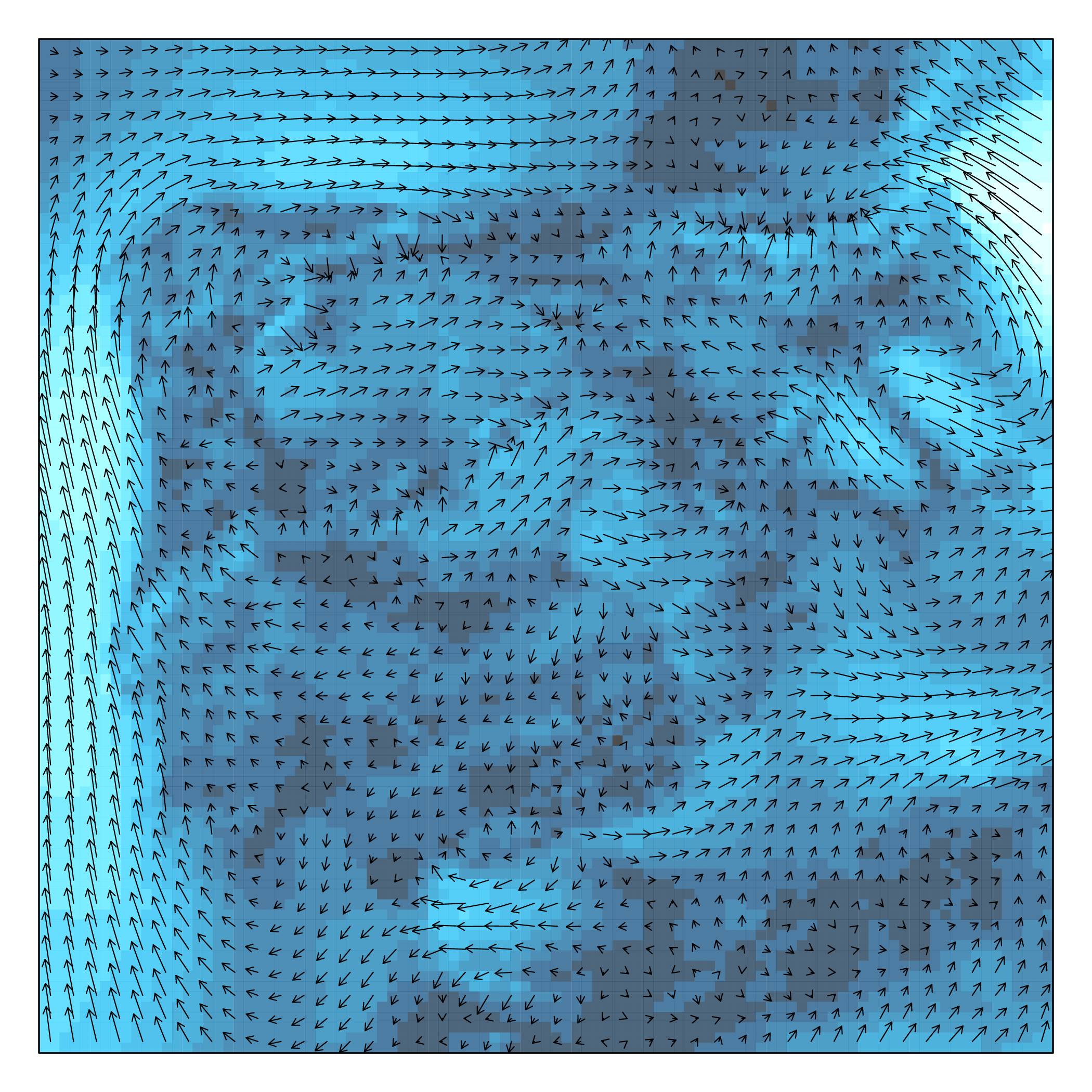
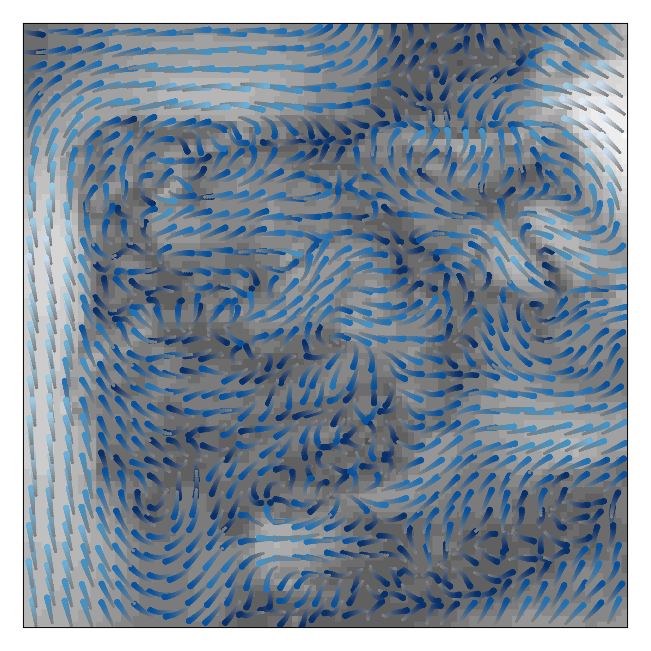
##################################################################
## Initial configuration
##################################################################
## Clone or download the repository and set the working directory
## with setwd to the folder where the repository is located.

library(raster)
library(rasterVis)

wDir <- raster('data/wDir')/180*pi
wSpeed <- raster('data/wSpeed')
windField <- stack(wSpeed, wDir)
names(windField) <- c('magnitude', 'direction')

##################################################################
## Arrow plot
##################################################################

vectorTheme <- BTCTheme(regions = list(alpha = 0.7))

vectorplot(windField, isField = TRUE,
           aspX = 5, aspY = 5,
           scaleSlope = FALSE,
           par.settings = vectorTheme,
           colorkey = FALSE,
           scales = list(draw = FALSE))

##################################################################
## Streamlines
##################################################################

myTheme <- streamTheme(
    region = rev(brewer.pal(n = 4, "Greys")),
    symbol = rev(brewer.pal(n = 9, "Blues")))

streamplot(windField, isField = TRUE,
           par.settings = myTheme,
           droplet = list(pc = 12),
           streamlet = list(L = 5, h = 5),
           scales = list(draw = FALSE),
           panel = panel.levelplot.raster)
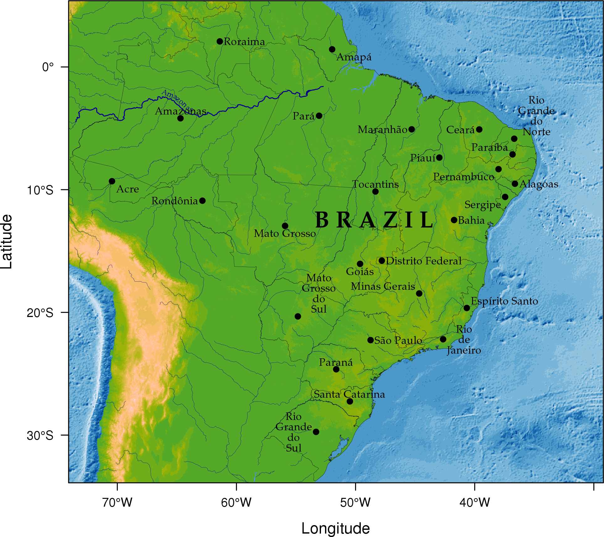
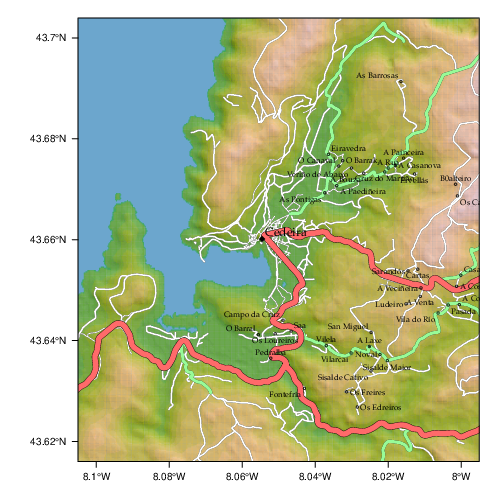
Physical maps
##################################################################
## Initial configuration
##################################################################
## Clone or download the repository and set the working directory
## with setwd to the folder where the repository is located.

##################################################################
## Physical maps
##################################################################

library(raster)
library(rasterVis)
library(rgdal)
library(rgeos)
library(latticeExtra)
library(colorspace)

##################################################################
## Retrieving data from DIVA-GIS, GADM and Natural Earth Data
##################################################################

     old <- setwd(tempdir())

     download.file('http://biogeo.ucdavis.edu/data/gadm2.8/shp/BRA_adm_shp.zip',
                   'BRA_adm.zip')
     unzip('BRA_adm.zip')
     brazilAdm <- readOGR(dsn = '.', layer = 'BRA_adm1')
     Encoding(levels(brazilAdm$NAME_1)) <- 'latin1'

     download.file('http://biogeo.ucdavis.edu/data/diva/alt/BRA_alt.zip',
                   'BRA_alt.zip')
     unzip('BRA_alt.zip')
     brazilDEM <- raster('BRA_alt')

     ## World Water lines (Natural Earth)
     download.file('http://www.naturalearthdata.com/http//www.naturalearthdata.com/download/10m/physical/ne_10m_rivers_lake_centerlines.zip',
                   'neRivers.zip')
     unzip('neRivers.zip')
     worldlRiv <- readOGR(dsn = '.', layer = 'ne_10m_rivers_lake_centerlines')

     download.file('http://www.naturalearthdata.com/http//www.naturalearthdata.com/download/10m/raster/OB_LR.zip',
                   'neSea.zip')
     unzip('neSea.zip')
     worldSea <- raster('OB_LR.tif')
     brazilSea <- crop(worldSea, brazilDEM)
     setwd(old)

##################################################################
## Intersection of shapefiles and elevation model
##################################################################

## only those features labeled as "River" are needed
worldRiv<- worldRiv[worldRiv$featurecla=='River',]

## Define the extent of Brazil as a SpatialPolygons
extBrazil <- as(extent(brazilDEM), 'SpatialPolygons')
proj4string(extBrazil) <- proj4string(worldRiv)

## and intersect it with worldRiv to extract brazilian rivers
## from the world database
brazilRiv <- gIntersection(worldRiv, extBrazil, byid=TRUE)
## and especially the famous Amazonas River
amazonas <- worldRiv[worldRiv$name=='Amazonas',]

##################################################################
## Labels
##################################################################

## Locations of labels of each polygon
centroids <- coordinates(brazilAdm)
## Location of the "Brazil" label (average of the set of polygons centroids)
xyBrazil <- apply(centroids, 2, mean)

admNames <- strsplit(as.character(brazilAdm$NAME_1), ' ')

admNames <- sapply(admNames,
                   FUN=function(s){
                       sep=if (length(s)>2) '\n' else  ' '
                       paste(s, collapse=sep)
                   })

##################################################################
## Overlaying layers of information
##################################################################

   blueTheme <- rasterTheme(region=brewer.pal(n=9, 'Blues'))

   seaPlot <- levelplot(brazilSea, par.settings=blueTheme,
                        maxpixels=1e6, panel=panel.levelplot.raster,
                        margin=FALSE, colorkey=FALSE)

  terrainTheme <- rasterTheme(region=terrain_hcl(15))

  altPlot <- levelplot(brazilDEM, par.settings=terrainTheme,
                       maxpixels=1e6, panel=panel.levelplot.raster,
                       margin=FALSE, colorkey=FALSE)

   amazonasLab <- label(amazonas, 'Amazonas')

  seaPlot + altPlot + layer({
      ## Rivers
      sp.lines(brazilRiv, col='darkblue', lwd=0.2)
      ## Amazonas
      sp.lineLabel(amazonas, amazonasLab,
                   lwd=1, col='darkblue', col.line='darkblue',
                   cex=0.5, fontfamily='Palatino')
      ## Administrative boundaries
      sp.polygons(brazilAdm, col='black', lwd=0.2)
      ## Centroids of administrative boundaries ...
      panel.points(centroids, col='black')
      ## ... with their labels
      panel.pointLabel(centroids, labels=admNames,
                       cex=0.7, fontfamily='Palatino', lineheight=.8)
      ## Country name
      panel.text(xyBrazil[1], xyBrazil[2], labels='B R A Z I L',
                 cex=1.5, fontfamily = 'Palatino', fontface=2)
  })

print(seaPlot, split=c(1, 1, 2, 1), more=TRUE)
print(altPlot, split=c(2, 1, 2, 1))
Data
##################################################################
## Initial configuration
##################################################################
## Clone or download the repository and set the working directory
## with setwd to the folder where the repository is located.

  ##################################################################
  ## Air Quality in Madrid
  ##################################################################

  ## codeStations.csv is extracted from the document
  ## http://www.mambiente.munimadrid.es/opencms/export/sites/default/calaire/Anexos/INTPHORA-DIA.pdf,
  ## table of page 3.

  codEstaciones <- read.csv2('data/codeStations.csv')
  codURL <- as.numeric(substr(codEstaciones$Codigo, 7, 8))

  ## The information of each measuring station is available at its own webpage, defined by codURL
  URLs <- paste('http://www.mambiente.munimadrid.es/opencms/opencms/calaire/contenidos/estaciones/estacion', codURL, '.html', sep = '')

##################################################################
## Data arrangement
##################################################################

  library(XML)
  library(sp)

  ## Access each webpage, retrieve tables and extract long/lat data
  coords <- lapply(URLs, function(est){
    tables <- readHTMLTable(est)
    location <- tables[[2]]
    ## Clean the table content and convert to dms format
    ub2dms <- function(x){
      ch <- as.character(x)
      ch <- sub(',', '.', ch)
      ch <- sub('O', 'W', ch) ## Some stations use "O" instead of "W"
      as.numeric(char2dms(ch, "º", "'", "'' "))
    }
    long <- ub2dms(location[2,1])
    lat <- ub2dms(location[2,2])
    alt <- as.numeric(sub(' m.', '', location[2, 3]))

    coords <- data.frame(long = long, lat = lat, alt = alt)

    coords
  })

  airStations <- cbind(codEstaciones, do.call(rbind, coords))

  ## The longitude of "El Pardo" station is wrong (positive instead of negative)
  airStations$long[22] <- -airStations$long[22]

  write.csv2(airStations, file = 'data/airStations.csv')

rawData <- readLines('data/Datos11.txt')
## This loop reads each line and extracts fields as defined by the
## INTPHORA file:
## http://www.mambiente.munimadrid.es/opencms/export/sites/default/calaire/Anexos/INTPHORA-DIA.pdf
datos11 <- lapply(rawData, function(x){
    codEst <- substr(x, 1, 8)
    codParam <- substr(x, 9, 10)
    codTec <- substr(x, 11, 12)
    codPeriod <- substr(x, 13, 14)
    month <- substr(x, 17, 18)
    dat <- substr(x, 19, nchar(x))
    ## "N" used for impossible days (31st April)
    idxN <- gregexpr('N', dat)[[1]]
    if (idxN==-1) idxN <- numeric(0)
    nZeroDays <- length(idxN)
    day <- seq(1, 31-nZeroDays)
    ## Substitute V and N with ";" to split data from different days
    dat <- gsub('[VN]+', ';', dat)
    dat <- as.numeric(strsplit(dat, ';')[[1]])
    ## Only data from valid days
    dat <- dat[day]
    res <- data.frame(codEst, codParam, ##codTec, codPeriod,
                      month, day, year = 2016,
                      dat)
})
datos11 <- do.call(rbind, datos11)

write.csv2(datos11, 'data/airQuality.csv')

##################################################################
## Combine data and spatial locations
##################################################################

  library(sp)

  ## Spatial location of stations
  airStations <- read.csv2('data/airStations.csv')
  coordinates(airStations) <- ~ long + lat
  ## Geographical projection
  proj4string(airStations) <- CRS("+proj=longlat +ellps=WGS84 +datum=WGS84")

  ## Measurements data
  airQuality <- read.csv2('data/airQuality.csv')
  ## Only interested in NO2
  NO2 <- airQuality[airQuality$codParam==8, ]

  NO2agg <- aggregate(dat ~ codEst, data = NO2,
                      FUN = function(x) {
                          c(mean = signif(mean(x), 3),
                            median = median(x),
                            sd = signif(sd(x), 3))
                          })
  NO2agg <- do.call(cbind, NO2agg)
  NO2agg <- as.data.frame(NO2agg)

library(rgdal)
library(maptools)
## Link aggregated data with stations to obtain a SpatialPointsDataFrame.
## Codigo and codEst are the stations codes
idxNO2 <- match(airStations$Codigo, NO2agg$codEst)
NO2sp <- spCbind(airStations[, c('Nombre', 'alt')], NO2agg[idxNO2, ])
## Save the result
writeOGR(NO2sp, dsn = 'data/', layer = 'NO2sp',
         driver = 'ESRI Shapefile')

##################################################################
## Photographs of the stations
##################################################################

library(XML)

old <- setwd('images')
for (i in 1:nrow(NO2df))
{
    codEst <- NO2df[i, "codEst"]
    ## Webpage of each station
    codURL <- as.numeric(substr(codEst, 7, 8))
    rootURL <- 'http://www.mambiente.munimadrid.es'
    stationURL <- paste(rootURL,
                        '/opencms/opencms/calaire/contenidos/estaciones/estacion',
                        codURL, '.html', sep = '')
    content <- htmlParse(stationURL, encoding = 'utf8')
    ## Extracted with http://www.selectorgadget.com/
    xPath <- '//*[contains(concat( " ", @class, " " ), concat( " ", "imagen_1", " " ))]'
    imageStation <- getNodeSet(content, xPath)[[1]]
    imageURL <- xmlAttrs(imageStation)[1]
    imageURL <- paste(rootURL, imageURL, sep = '')
    download.file(imageURL, destfile = paste(codEst, '.jpg', sep = ''))
}
setwd(old)

##################################################################
## Spanish General Elections
##################################################################

dat2016 <- read.csv('data/GeneralSpanishElections2016.csv')

census <- dat2016$Total.censo.electoral
validVotes <- dat2016$Votos.válidos
## Election results per political party and municipality
votesData <- dat2016[, -(1:13)]
## Abstention as an additional party
votesData$ABS <- census - validVotes
## UP is a coalition of several parties
UPcols <- grep("PODEMOS|ECP", names(votesData))
votesData$UP <- rowSums(votesData[, UPcols])
votesData[, UPcols] <- NULL
## Winner party at each municipality
whichMax <- apply(votesData,  1, function(x)names(votesData)[which.max(x)])
## Results of the winner party at each municipality
Max <- apply(votesData, 1, max)
## OTH for everything but PP, PSOE, UP, Cs, and ABS
whichMax[!(whichMax %in% c('PP', 'PSOE', 'UP', 'C.s', 'ABS'))] <- 'OTH'
## Percentage of votes with the electoral census
pcMax <- Max/census * 100

## Province-Municipality code. sprintf formats a number with leading zeros.
PROVMUN <- with(dat2016, paste(sprintf('%02d', Código.de.Provincia),
                               sprintf('%03d', Código.de.Municipio),
                               sep=""))

votes2016 <- data.frame(PROVMUN, whichMax, Max, pcMax)
write.csv(votes2016, 'data/votes2016.csv', row.names = FALSE)

##################################################################
## Administrative boundaries
##################################################################

library(sp)
library(rgdal)

old <- setwd(tempdir())

download.file('ftp://www.ine.es/pcaxis/mapas_completo_municipal.rar',
              'mapas_completo_municipal.rar')
system2('unrar', c('e', 'mapas_completo_municipal.rar'))

spMap <- readOGR("esp_muni_0109.shp",
                 p4s = "+proj=utm +zone=30 +ellps=GRS80 +units=m +no_defs")
Encoding(levels(spMap$NOMBRE)) <- "latin1"

setwd(old)

## dissolve repeated polygons
spPols <- unionSpatialPolygons(spMap, spMap$PROVMUN)

votes2016 <- read.csv('data/votes2016.csv',
                        colClasses = c('factor', 'factor', 'numeric', 'numeric'))

## Match polygons and data using ID slot and PROVMUN column
IDs <- sapply(spPols@polygons, function(x)x@ID)
idx <- match(IDs, votes2016$PROVMUN)

##Places without information
idxNA <- which(is.na(idx))

##Information to be added to the SpatialPolygons object
dat2add <- votes2016[idx, ]

## SpatialPolygonsDataFrame uses row names to match polygons with data
row.names(dat2add) <- IDs
spMapVotes <- SpatialPolygonsDataFrame(spPols, dat2add)

## Drop those places without information
spMapVotes0 <- spMapVotes[-idxNA, ]

## Save the result
writeOGR(spMapVotes0, dsn = 'data/', layer = 'spMapVotes0',
         drive = 'ESRI Shapefile')

## Extract Canarias islands from the SpatialPolygons object
canarias <-  sapply(spMapVotes0@polygons, function(x)substr(x@ID, 1, 2) %in% c("35",  "38"))
peninsula <- spMapVotes0[!canarias,]
island <- spMapVotes0[canarias,]

## Shift the island extent box to position them at the bottom right corner
dy <- bbox(peninsula)[2,1] - bbox(island)[2,1]
dx <- bbox(peninsula)[1,2] - bbox(island)[1,2]
island2 <- elide(island, shift = c(dx, dy))
bbIslands <- bbox(island2)
proj4string(island2) <- proj4string(peninsula)

## Bind Peninsula (without islands) with shifted islands
spMapVotes <- rbind(peninsula, island2)

## Save the result
writeOGR(spMapVotes, dsn = 'data/', layer = 'spMapVotes',
         drive = 'ESRI Shapefile')

  ##################################################################
  ## CM SAF
  ##################################################################

  library(raster)

  tmp <- tempdir()
  unzip('data/SISmm2008_CMSAF.zip', exdir = tmp)
  filesCMSAF <- dir(tmp, pattern = 'SISmm')
  SISmm <- stack(paste(tmp, filesCMSAF, sep = '/'))
  ## CM-SAF data is average daily irradiance (W/m2). Multiply by 24
  ## hours to obtain daily irradiation (Wh/m2)
  SISmm <- SISmm * 24

  ## Monthly irradiation: each month by the corresponding number of days
  daysMonth <- c(31, 29, 31, 30, 31, 30, 31, 31, 30, 31, 30, 31)
  SISm <- SISmm * daysMonth / 1000 ## kWh/m2
  ## Annual average
  SISav <- sum(SISm)/sum(daysMonth)
  writeRaster(SISav, file = 'SISav')

 library(raster)
 ## http://neo.sci.gsfc.nasa.gov/Search.html?group=64
 pop <- raster('875430rgb-167772161.0.FLOAT.TIFF')
 ## http://neo.sci.gsfc.nasa.gov/Search.html?group=20
 landClass <- raster('241243rgb-167772161.0.TIFF')