Estadística básica con R

Índice

1. Conjunto de datos
2. Estadística Univariante
3. Generar datos aleatorios
4. Tests de Hipótesis
5. Regresión lineal

1 Conjunto de datos

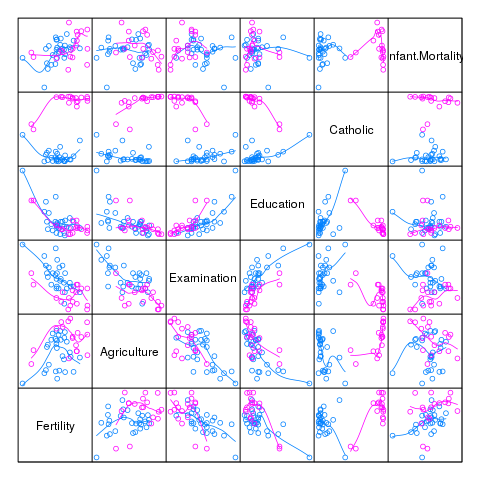
1.1 Conjunto de datos: swiss

Standardized fertility measure and socio-economic indicators for each of 47 French-speaking provinces of Switzerland at about 1888. 6 variables in percent [0, 100]:

Fertility: Ig, ‘common standardized fertility measure’
Agriculture: % of males involved in agriculture as occupation
Examination: % draftees receiving highest mark on army examination
Education: % education beyond primary school for draftees.
Catholic: % ‘catholic’ (as opposed to ‘protestant’).
Infant.Mortality: live births who live less than 1year.

1.2 Conjunto de datos: swiss

data(swiss)

summary(swiss)

   Fertility      Agriculture     Examination      Education    
 Min.   :35.00   Min.   : 1.20   Min.   : 3.00   Min.   : 1.00  
 1st Qu.:64.70   1st Qu.:35.90   1st Qu.:12.00   1st Qu.: 6.00  
 Median :70.40   Median :54.10   Median :16.00   Median : 8.00  
 Mean   :70.14   Mean   :50.66   Mean   :16.49   Mean   :10.98  
 3rd Qu.:78.45   3rd Qu.:67.65   3rd Qu.:22.00   3rd Qu.:12.00  
 Max.   :92.50   Max.   :89.70   Max.   :37.00   Max.   :53.00  
    Catholic       Infant.Mortality
 Min.   :  2.150   Min.   :10.80   
 1st Qu.:  5.195   1st Qu.:18.15   
 Median : 15.140   Median :20.00   
 Mean   : 41.144   Mean   :19.94   
 3rd Qu.: 93.125   3rd Qu.:21.70   
 Max.   :100.000   Max.   :26.60

1.3

library(lattice)
splom(swiss, pscale=0, type=c('p', 'smooth'),
      groups=swiss$Catholic > 50, xlab='')

2 Estadística Univariante

2.1 Resumen de información

summary(swiss)

   Fertility      Agriculture     Examination      Education    
 Min.   :35.00   Min.   : 1.20   Min.   : 3.00   Min.   : 1.00  
 1st Qu.:64.70   1st Qu.:35.90   1st Qu.:12.00   1st Qu.: 6.00  
 Median :70.40   Median :54.10   Median :16.00   Median : 8.00  
 Mean   :70.14   Mean   :50.66   Mean   :16.49   Mean   :10.98  
 3rd Qu.:78.45   3rd Qu.:67.65   3rd Qu.:22.00   3rd Qu.:12.00  
 Max.   :92.50   Max.   :89.70   Max.   :37.00   Max.   :53.00  
    Catholic       Infant.Mortality
 Min.   :  2.150   Min.   :10.80   
 1st Qu.:  5.195   1st Qu.:18.15   
 Median : 15.140   Median :20.00   
 Mean   : 41.144   Mean   :19.94   
 3rd Qu.: 93.125   3rd Qu.:21.70   
 Max.   :100.000   Max.   :26.60

2.2 Media

mean(swiss$Fertility)

[1] 70.14255

colMeans(swiss)

Fertility      Agriculture      Examination        Education 
 70.14255         50.65957         16.48936         10.97872 
 Catholic Infant.Mortality 
 41.14383         19.94255

2.3 Desviación Estándar

sd(swiss$Fertility)

[1] 12.4917

sapply(swiss, sd)

Fertility      Agriculture      Examination        Education 
12.491697        22.711218         7.977883         9.615407 
 Catholic Infant.Mortality 
41.704850         2.912697

2.4 Otras

median(swiss$Fertility)

[1] 70.4

mad(swiss$Fertility)

[1] 10.22994

IQR(swiss$Fertility)

[1] 13.75

3 Generar datos aleatorios

3.1 Distribuciones disponibles

BMCOL
- beta beta
- binomial binom
- Cauchy cauchy
- chi-squared chisq
- exponential exp
- F f
- gamma gamma
- geometric geom
- hypergeometric hyper
BMCOL
- log-normal lnorm
- logistic logis
- negative binomial
- normal norm
- Poisson pois
- signed rank signrank
- Student’s t t
- uniform unif
- Weibull weibull
- Wilcoxon wilcox

3.2 Densidad, CDF, Cuantiles, y Números aleatorios

dxxx: función de densidad de probabilidad
pxxx: función acumulada de probabilidad
qxxx: cuantiles
rxxx: generación de números aleatorios

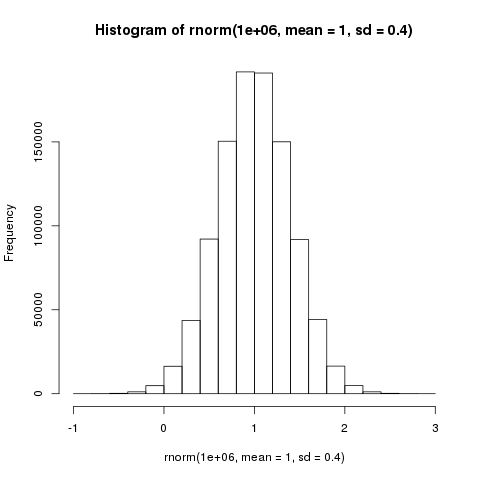
3.3 Distribución Normal

rnorm(10, mean = 1, sd = .4)

[1] 0.5987165 0.7374486 1.0635955 0.2232172 1.0509421 0.9659542 0.5948662
[8] 0.8766249 1.0982419 0.9985146

hist(rnorm(1e6, mean = 1, sd = .4))

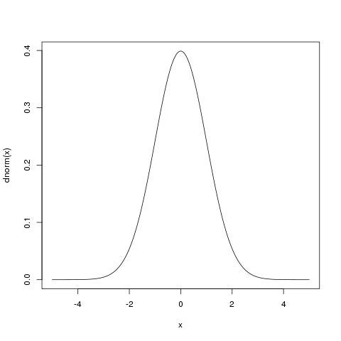
3.4 Distribución Normal

x <- seq( -5, 5, by =.01)
plot(x, dnorm(x), type = 'l')

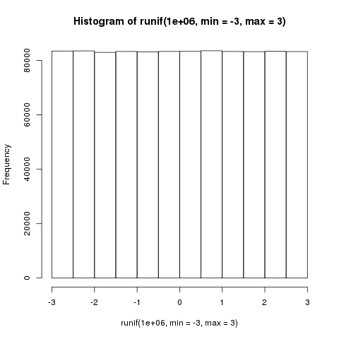
3.5 Distribución Uniforme

runif(10, min=-3, max=3)

[1]  1.2153711 -2.8451359  0.8235075 -1.0147079 -1.7177479 -1.3571362
[7]  2.7228768  0.2771958  0.7458442 -1.8732231

hist(runif(1e6, min = -3, max = 3))

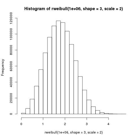
3.6 Distribución de Weibull

rweibull(n=10, shape = 3, scale = 2)

[1] 0.7661914 1.3502844 0.9237997 1.8538150 1.8644202 2.5229566 1.6498369
[8] 1.8534614 1.9982788 2.7837383

hist(rweibull(1e6, shape = 3, scale = 2))

3.7 Muestreo aleatorio

x <- seq(1, 100, length = 10)
x

[1]   1  12  23  34  45  56  67  78  89 100

Sin reemplazo

sample(x)

[1]  12  23  45  78   1 100  34  89  67  56

sample(x, 5)

[1]  89 100  56  23  12

Con reemplazo

sample(x, 5, replace = TRUE)

[1]  1 56 89 45 89

4 Tests de Hipótesis

4.1 Para muestra única

t de Student

t.test(swiss$Fertility, mu=70)

	One Sample t-test

data:  swiss$Fertility
t = 0.078236, df = 46, p-value = 0.938
alternative hypothesis: true mean is not equal to 70
95 percent confidence interval:
 66.47485 73.81025
sample estimates:
mean of x 
 70.14255

Wilcoxon (no paramétrico)

wilcox.test(swiss$Fertility, mu=70)

	Wilcoxon signed rank test with continuity correction

data:  swiss$Fertility
V = 592.5, p-value = 0.767
alternative hypothesis: true location is not equal to 70

Warning message:
In wilcox.test.default(swiss$Fertility, mu = 70) :
  cannot compute exact p-value with ties

4.2 Para muestras pareadas

Religion <- ifelse(swiss$Catholic > 50,
                   'Catholic', 'Protestant')

t de Student

t.test(Fertility ~ Religion, data=swiss)

	Welch Two Sample t-test

data:  Fertility by Religion
t = 2.7004, df = 26.742, p-value = 0.01186
alternative hypothesis: true difference in means is not equal to 0
95 percent confidence interval:
  2.455904 18.024939
sample estimates:
  mean in group Catholic mean in group Protestant 
                76.46111                 66.22069

4.3 Para muestras pareadas

Wilcoxon

wilcox.test(Fertility ~ Religion, data=swiss)

	Wilcoxon rank sum test with continuity correction

data:  Fertility by Religion
W = 409.5, p-value = 0.0012
alternative hypothesis: true location shift is not equal to 0

Warning message:
In wilcox.test.default(x = c(83.1, 92.5, 76.1, 83.8, 92.4, 82.4,  :
  cannot compute exact p-value with ties

5 Regresión lineal

5.1 Fertilidad y educación

lmFertEdu <- lm(Fertility ~ Education,
              data = swiss)
summary(lmFertEdu)

Call:
lm(formula = Fertility ~ Education, data = swiss)

Residuals:
    Min      1Q  Median      3Q     Max 
-17.036  -6.711  -1.011   9.526  19.689 

Coefficients:
            Estimate Std. Error t value Pr(>|t|)    
(Intercept)  79.6101     2.1041  37.836  < 2e-16 ***
Education    -0.8624     0.1448  -5.954 3.66e-07 ***
---
Signif. codes:  0 ‘***’ 0.001 ‘**’ 0.01 ‘*’ 0.05 ‘.’ 0.1 ‘ ’ 1

Residual standard error: 9.446 on 45 degrees of freedom
Multiple R-squared:  0.4406,	Adjusted R-squared:  0.4282 
F-statistic: 35.45 on 1 and 45 DF,  p-value: 3.659e-07

5.2 Fertilidad y educación

coef(lmFertEdu)

(Intercept)   Education 
 79.6100585  -0.8623503

fitted.values(lmFertEdu)

  Courtelary     Delemont Franches-Mnt      Moutier   Neuveville   Porrentruy 
    69.26186     71.84891     75.29831     73.57361     66.67480     73.57361 
       Broye        Glane      Gruyere       Sarine      Veveyse        Aigle 
    73.57361     72.71126     73.57361     68.39950     74.43596     69.26186 
     Aubonne     Avenches     Cossonay    Echallens     Grandson     Lausanne 
    73.57361     69.26186     75.29831     77.88536     72.71126     55.46425 
   La Vallee       Lavaux       Morges       Moudon        Nyone         Orbe 
    62.36305     71.84891     70.98656     77.02301     69.26186     74.43596 
        Oron      Payerne Paysd'enhaut        Rolle        Vevey      Yverdon 
    78.74771     72.71126     77.02301     70.98656     63.22540     72.71126 
     Conthey    Entremont       Herens     Martigwy      Monthey   St Maurice 
    77.88536     74.43596     77.88536     74.43596     77.02301     71.84891 
      Sierre         Sion       Boudry La Chauxdfnd     Le Locle    Neuchatel 
    77.02301     68.39950     69.26186     70.12421     68.39950     52.01485 
  Val de Ruz ValdeTravers V. De Geneve  Rive Droite  Rive Gauche 
    73.57361     73.57361     33.90549     54.60190     54.60190

5.3 Fertilidad y educación

residuals(lmFertEdu)

  Courtelary     Delemont Franches-Mnt      Moutier   Neuveville   Porrentruy 
  10.9381450   11.2510941   17.2016929   12.2263935   10.2251959    2.5263935 
       Broye        Glane      Gruyere       Sarine      Veveyse        Aigle 
  10.2263935   19.6887438    8.8263935   14.5004953   12.6640432   -5.1618550 
     Aubonne     Avenches     Cossonay    Echallens     Grandson     Lausanne 
  -6.6736065   -0.3618550  -13.5983071   -9.5853579   -1.0112562    0.2357497 
   La Vallee       Lavaux       Morges       Moudon        Nyone         Orbe 
  -8.0630527   -6.7489059   -5.4865556  -12.0230077  -12.6618550  -17.0359568 
        Oron      Payerne Paysd'enhaut        Rolle        Vevey      Yverdon 
  -6.2477082    1.4887438   -5.0230077  -10.4865556   -4.9254030   -7.3112562 
     Conthey    Entremont       Herens     Martigwy      Monthey   St Maurice 
  -2.3853579   -5.1359568   -0.5853579   -3.9359568    2.3769923   -6.8489059 
      Sierre         Sion       Boudry La Chauxdfnd     Le Locle    Neuchatel 
  15.1769923   10.9004953    1.1381450   -4.4242053    4.3004953   12.3851508 
  Val de Ruz ValdeTravers V. De Geneve  Rive Droite  Rive Gauche 
   4.0263935   -5.9736065    1.0945070   -9.9019000  -11.8019000

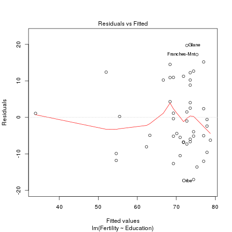
5.4 Fertilidad y educación

plot(lmFertEdu, which = 1)

5.5 Fertilidad, educación y religión

lmFertEduCat <- lm(Fertility ~ Education + Catholic,
                   data = swiss)
summary(lmFertEduCat)

Call:
lm(formula = Fertility ~ Education + Catholic, data = swiss)

Residuals:
    Min      1Q  Median      3Q     Max 
-15.042  -6.578  -1.431   6.122  14.322 

Coefficients:
            Estimate Std. Error t value Pr(>|t|)    
(Intercept) 74.23369    2.35197  31.562  < 2e-16 ***
Education   -0.78833    0.12929  -6.097 2.43e-07 ***
Catholic     0.11092    0.02981   3.721  0.00056 ***
---
Signif. codes:  0 ‘***’ 0.001 ‘**’ 0.01 ‘*’ 0.05 ‘.’ 0.1 ‘ ’ 1

Residual standard error: 8.331 on 44 degrees of freedom
Multiple R-squared:  0.5745,	Adjusted R-squared:  0.5552 
F-statistic:  29.7 on 2 and 44 DF,  p-value: 6.849e-09

5.6 Lo mismo con `update`

lmFertEduCat <- update(lmFertEdu, . ~ . + Catholic,
                       data = swiss)
summary(lmFertEduCat)

Call:
lm(formula = Fertility ~ Education + Catholic, data = swiss)

Residuals:
    Min      1Q  Median      3Q     Max 
-15.042  -6.578  -1.431   6.122  14.322 

Coefficients:
            Estimate Std. Error t value Pr(>|t|)    
(Intercept) 74.23369    2.35197  31.562  < 2e-16 ***
Education   -0.78833    0.12929  -6.097 2.43e-07 ***
Catholic     0.11092    0.02981   3.721  0.00056 ***
---
Signif. codes:  0 ‘***’ 0.001 ‘**’ 0.01 ‘*’ 0.05 ‘.’ 0.1 ‘ ’ 1

Residual standard error: 8.331 on 44 degrees of freedom
Multiple R-squared:  0.5745,	Adjusted R-squared:  0.5552 
F-statistic:  29.7 on 2 and 44 DF,  p-value: 6.849e-09

5.7 Fertilidad, educación, religión y agricultura

lmFertEduCatAgr <- lm(Fertility ~ Education + Catholic + Agriculture,
                      data = swiss)
summary(lmFertEduCatAgr)

Call:
lm(formula = Fertility ~ Education + Catholic + Agriculture, 
    data = swiss)

Residuals:
    Min      1Q  Median      3Q     Max 
-15.178  -6.548   1.379   5.822  14.840 

Coefficients:
            Estimate Std. Error t value Pr(>|t|)    
(Intercept) 86.22502    4.73472  18.211  < 2e-16 ***
Education   -1.07215    0.15580  -6.881 1.91e-08 ***
Catholic     0.14520    0.03015   4.817 1.84e-05 ***
Agriculture -0.20304    0.07115  -2.854  0.00662 ** 
---
Signif. codes:  0 ‘***’ 0.001 ‘**’ 0.01 ‘*’ 0.05 ‘.’ 0.1 ‘ ’ 1

Residual standard error: 7.728 on 43 degrees of freedom
Multiple R-squared:  0.6423,	Adjusted R-squared:  0.6173 
F-statistic: 25.73 on 3 and 43 DF,  p-value: 1.089e-09

5.8 Lo mismo con `update`

lmFertEduCatAgr <- update(lmFertEduCat,
                          . ~ . + Agriculture,
                          data = swiss)
summary(lmFertEduCatAgr)

Call:
lm(formula = Fertility ~ Education + Catholic + Agriculture, 
    data = swiss)

Residuals:
    Min      1Q  Median      3Q     Max 
-15.178  -6.548   1.379   5.822  14.840 

Coefficients:
            Estimate Std. Error t value Pr(>|t|)    
(Intercept) 86.22502    4.73472  18.211  < 2e-16 ***
Education   -1.07215    0.15580  -6.881 1.91e-08 ***
Catholic     0.14520    0.03015   4.817 1.84e-05 ***
Agriculture -0.20304    0.07115  -2.854  0.00662 ** 
---
Signif. codes:  0 ‘***’ 0.001 ‘**’ 0.01 ‘*’ 0.05 ‘.’ 0.1 ‘ ’ 1

Residual standard error: 7.728 on 43 degrees of freedom
Multiple R-squared:  0.6423,	Adjusted R-squared:  0.6173 
F-statistic: 25.73 on 3 and 43 DF,  p-value: 1.089e-09

5.9 Lo mismo con `update`

lmFertEduCatAgr <- update(lmFertEdu,
                          . ~ . + Catholic + Agriculture,
                          data = swiss)
summary(lmFertEduCatAgr)

Call:
lm(formula = Fertility ~ Education + Catholic + Agriculture, 
    data = swiss)

Residuals:
    Min      1Q  Median      3Q     Max 
-15.178  -6.548   1.379   5.822  14.840 

Coefficients:
            Estimate Std. Error t value Pr(>|t|)    
(Intercept) 86.22502    4.73472  18.211  < 2e-16 ***
Education   -1.07215    0.15580  -6.881 1.91e-08 ***
Catholic     0.14520    0.03015   4.817 1.84e-05 ***
Agriculture -0.20304    0.07115  -2.854  0.00662 ** 
---
Signif. codes:  0 ‘***’ 0.001 ‘**’ 0.01 ‘*’ 0.05 ‘.’ 0.1 ‘ ’ 1

Residual standard error: 7.728 on 43 degrees of freedom
Multiple R-squared:  0.6423,	Adjusted R-squared:  0.6173 
F-statistic: 25.73 on 3 and 43 DF,  p-value: 1.089e-09

5.10 Comparamos modelos con `anova`

anova(lmFertEdu, lmFertEduCat, lmFertEduCatAgr)

Analysis of Variance Table

Model 1: Fertility ~ Education
Model 2: Fertility ~ Education + Catholic
Model 3: Fertility ~ Education + Catholic + Agriculture
  Res.Df    RSS Df Sum of Sq      F    Pr(>F)    
1     45 4015.2                                  
2     44 3054.2  1    961.07 16.093 0.0002365 ***
3     43 2567.9  1    486.28  8.143 0.0066235 ** 
---
Signif. codes:  0 ‘***’ 0.001 ‘**’ 0.01 ‘*’ 0.05 ‘.’ 0.1 ‘ ’ 1

5.11 Fertilidad contra todo

lmFert <- lm(Fertility ~ ., data=swiss)

summary(lmFert)

Call:
lm(formula = Fertility ~ ., data = swiss)

Residuals:
     Min       1Q   Median       3Q      Max 
-15.2743  -5.2617   0.5032   4.1198  15.3213 

Coefficients:
                 Estimate Std. Error t value Pr(>|t|)    
(Intercept)      66.91518   10.70604   6.250 1.91e-07 ***
Agriculture      -0.17211    0.07030  -2.448  0.01873 *  
Examination      -0.25801    0.25388  -1.016  0.31546    
Education        -0.87094    0.18303  -4.758 2.43e-05 ***
Catholic          0.10412    0.03526   2.953  0.00519 ** 
Infant.Mortality  1.07705    0.38172   2.822  0.00734 ** 
---
Signif. codes:  0 ‘***’ 0.001 ‘**’ 0.01 ‘*’ 0.05 ‘.’ 0.1 ‘ ’ 1

Residual standard error: 7.165 on 41 degrees of freedom
Multiple R-squared:  0.7067,	Adjusted R-squared:  0.671 
F-statistic: 19.76 on 5 and 41 DF,  p-value: 5.594e-10

5.12 Elegir un modelo con `anova`

anova(lmFert)

Analysis of Variance Table

Response: Fertility
                 Df  Sum Sq Mean Sq F value    Pr(>F)    
Agriculture       1  894.84  894.84 17.4288 0.0001515 ***
Examination       1 2210.38 2210.38 43.0516 6.885e-08 ***
Education         1  891.81  891.81 17.3699 0.0001549 ***
Catholic          1  667.13  667.13 12.9937 0.0008387 ***
Infant.Mortality  1  408.75  408.75  7.9612 0.0073357 ** 
Residuals        41 2105.04   51.34                      
---
Signif. codes:  0 ‘***’ 0.001 ‘**’ 0.01 ‘*’ 0.05 ‘.’ 0.1 ‘ ’ 1

5.13 Elegir un modelo con `step`

stepFert <- step(lmFert)

Start:  AIC=190.69
Fertility ~ Agriculture + Examination + Education + Catholic + 
    Infant.Mortality

                   Df Sum of Sq    RSS    AIC
- Examination       1     53.03 2158.1 189.86
<none>                          2105.0 190.69
- Agriculture       1    307.72 2412.8 195.10
- Infant.Mortality  1    408.75 2513.8 197.03
- Catholic          1    447.71 2552.8 197.75
- Education         1   1162.56 3267.6 209.36

Step:  AIC=189.86
Fertility ~ Agriculture + Education + Catholic + Infant.Mortality

                   Df Sum of Sq    RSS    AIC
<none>                          2158.1 189.86
- Agriculture       1    264.18 2422.2 193.29
- Infant.Mortality  1    409.81 2567.9 196.03
- Catholic          1    956.57 3114.6 205.10
- Education         1   2249.97 4408.0 221.43

5.14 Elegir un modelo

summary(stepFert)

Call:
lm(formula = Fertility ~ Agriculture + Education + Catholic + 
    Infant.Mortality, data = swiss)

Residuals:
     Min       1Q   Median       3Q      Max 
-14.6765  -6.0522   0.7514   3.1664  16.1422 

Coefficients:
                 Estimate Std. Error t value Pr(>|t|)    
(Intercept)      62.10131    9.60489   6.466 8.49e-08 ***
Agriculture      -0.15462    0.06819  -2.267  0.02857 *  
Education        -0.98026    0.14814  -6.617 5.14e-08 ***
Catholic          0.12467    0.02889   4.315 9.50e-05 ***
Infant.Mortality  1.07844    0.38187   2.824  0.00722 ** 
---
Signif. codes:  0 ‘***’ 0.001 ‘**’ 0.01 ‘*’ 0.05 ‘.’ 0.1 ‘ ’ 1

Residual standard error: 7.168 on 42 degrees of freedom
Multiple R-squared:  0.6993,	Adjusted R-squared:  0.6707 
F-statistic: 24.42 on 4 and 42 DF,  p-value: 1.717e-10

5.15 Elegir un modelo

stepFert$anova

           Step Df Deviance Resid. Df Resid. Dev      AIC
1               NA       NA        41   2105.043 190.6913
2 - Examination  1 53.02656        42   2158.069 189.8606

Estadística básica con R

Índice

1 Conjunto de datos

1.1 Conjunto de datos: swiss

1.2 Conjunto de datos: swiss

1.3

2 Estadística Univariante

2.1 Resumen de información

2.2 Media

2.3 Desviación Estándar

2.4 Otras

3 Generar datos aleatorios

3.1 Distribuciones disponibles

3.2 Densidad, CDF, Cuantiles, y Números aleatorios

3.3 Distribución Normal

3.4 Distribución Normal

3.5 Distribución Uniforme

3.6 Distribución de Weibull

3.7 Muestreo aleatorio

4 Tests de Hipótesis

4.1 Para muestra única

4.2 Para muestras pareadas

4.3 Para muestras pareadas

5 Regresión lineal

5.1 Fertilidad y educación

5.2 Fertilidad y educación

5.3 Fertilidad y educación

5.4 Fertilidad y educación

5.5 Fertilidad, educación y religión

5.6 Lo mismo con update

5.7 Fertilidad, educación, religión y agricultura

5.8 Lo mismo con update

5.9 Lo mismo con update

5.10 Comparamos modelos con anova

5.11 Fertilidad contra todo

5.12 Elegir un modelo con anova

5.13 Elegir un modelo con step

5.14 Elegir un modelo

5.15 Elegir un modelo

5.6 Lo mismo con `update`

5.8 Lo mismo con `update`

5.9 Lo mismo con `update`

5.10 Comparamos modelos con `anova`

5.12 Elegir un modelo con `anova`

5.13 Elegir un modelo con `step`