Spatio-temporal data - Displaying time series, spatial and space-time data with R
Table of Contents
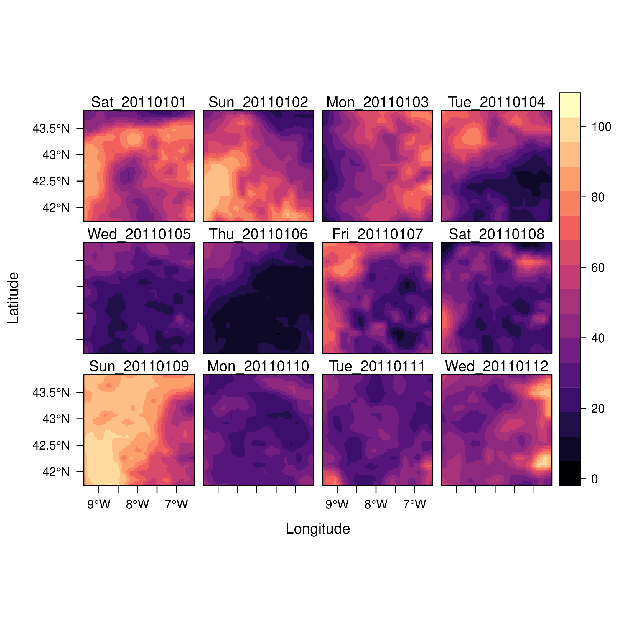
Raster data
Level plots
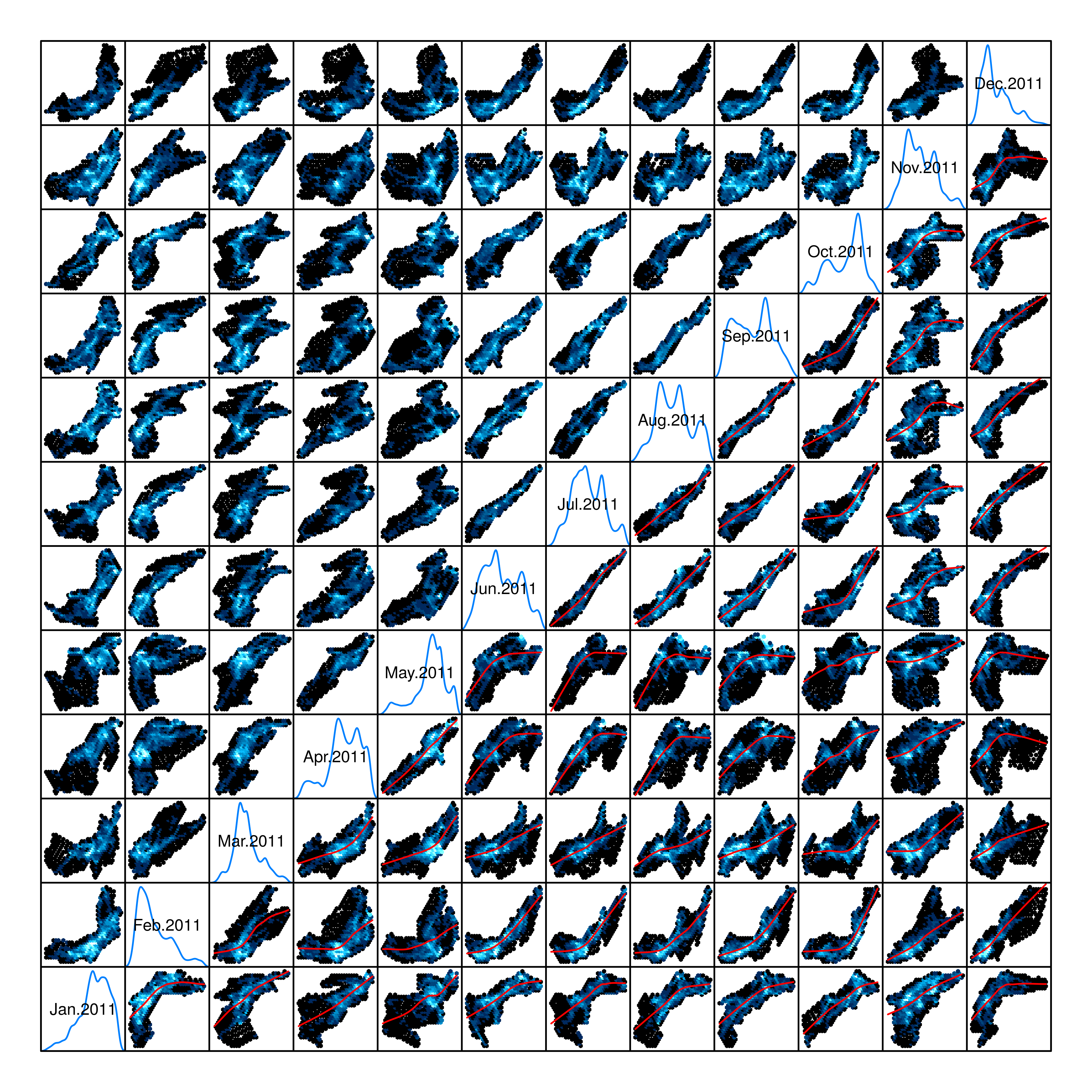
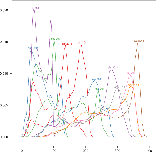
Graphical Exploratory Data Analysis

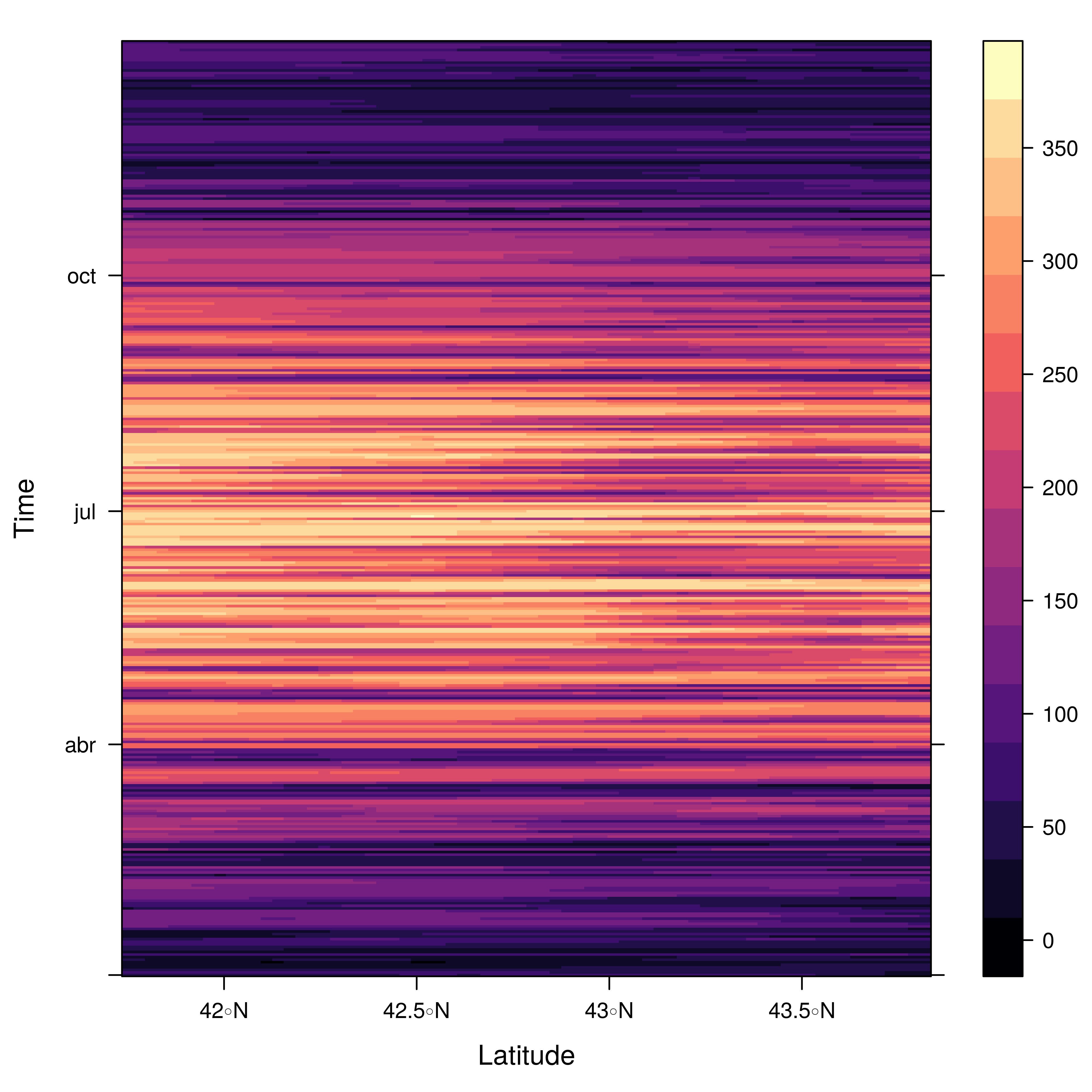
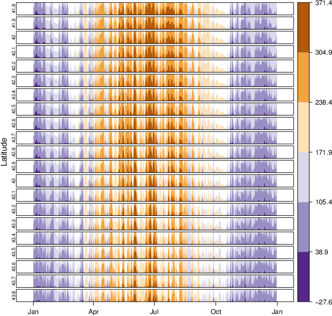
Space-Time and Time Series Plots
Spatial point data
Graphics with spacetime


Animation


Code
Raster data
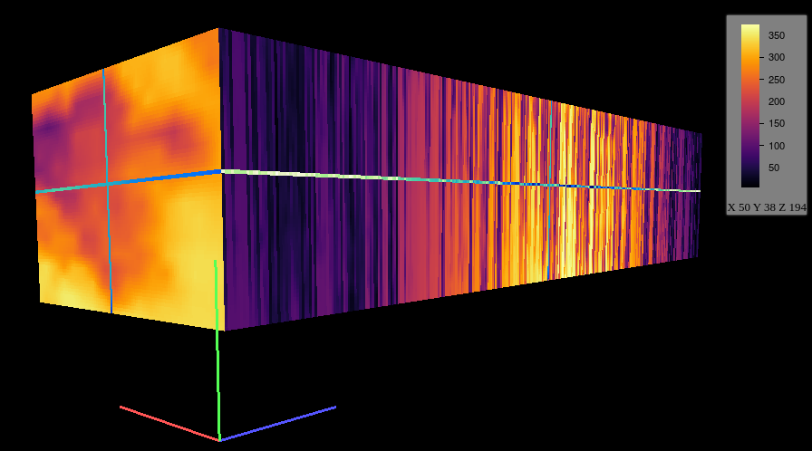
##################################################################
## Initial configuration
##################################################################
## Clone or download the repository and set the working directory
## with setwd to the folder where the repository is located.

Sys.setlocale("LC_TIME", 'C')

##################################################################
## CMSAF Data
##################################################################

library(raster)
library(zoo)
library(rasterVis)

SISdm <- brick('data/SISgal')

timeIndex <- seq(as.Date('2011-01-01'), by = 'day', length = 365)
SISdm <- setZ(SISdm, timeIndex)
names(SISdm) <- format(timeIndex, '%a_%Y%m%d')

##################################################################
## Levelplot
##################################################################

levelplot(SISdm, layers = 1:12, panel = panel.levelplot.raster)

SISmm <- zApply(SISdm, by = as.yearmon, fun = 'mean')

levelplot(SISmm, panel = panel.levelplot.raster)

##################################################################
## Exploratory graphics
##################################################################

histogram(SISdm, FUN = as.yearmon)

bwplot(SISdm, FUN = as.yearmon)

splom(SISmm, xlab = '', plot.loess = TRUE)

##################################################################
## Space-time and time series plots
##################################################################

hovmoller(SISdm)

xyplot(SISdm, auto.key = list(space = 'right'))

horizonplot(SISdm, digits = 1,
            col.regions = rev(brewer.pal(n = 6, 'PuOr')),
            xlab = '', ylab = 'Latitude')

library(mapview)

cubeView(SISdm)
Spatial point data
##################################################################
## Initial configuration
##################################################################
## Clone or download the repository and set the working directory
## with setwd to the folder where the repository is located.

library(lattice)
library(latticeExtra)

Sys.setlocale("LC_TIME", 'C')

source('configLattice.R')

##################################################################
## Data and spatial information
##################################################################

library(sp)

## Spatial location of stations
airStations <- read.csv2('data/airStations.csv')
## rownames are used as the ID of the Spatial object
rownames(airStations) <- substring(airStations$Codigo, 7)
coordinates(airStations) <- ~ long + lat
proj4string(airStations) <- CRS("+proj=longlat +ellps=WGS84")
## Measurements data
airQuality <- read.csv2('data/airQuality.csv')
## Only interested in NO2
NO2 <- airQuality[airQuality$codParam == 8, ]

library(zoo)
library(reshape2)
library(spacetime)

NO2$time <- as.Date(with(NO2,
                         ISOdate(year, month, day)))

NO2wide <- dcast(NO2[, c('codEst', 'dat', 'time')],
                 time ~ codEst,
                 value.var = "dat")

NO2zoo <- zoo(NO2wide[,-1], NO2wide$time)

dats <- data.frame(vals = as.vector(t(NO2zoo)))

NO2st <- STFDF(sp = airStations,
               time = index(NO2zoo),
               data = dats)

##################################################################
## Graphics with spacetime
##################################################################

airPal <- colorRampPalette(c('springgreen1', 'sienna3', 'gray5'))(5)

stplot(NO2st[, 1:12],
       cuts = 5,
       col.regions = airPal,
       main = '',
       edge.col = 'black')

stplot(NO2st, mode = 'xt',
       col.regions = colorRampPalette(airPal)(15),
       scales = list(x = list(rot = 45)),
       ylab = '', xlab = '', main = '')

stplot(NO2st, mode = 'ts',
       xlab = '',
       lwd = 0.1, col = 'black', alpha = 0.6,
       auto.key = FALSE)
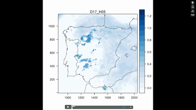
Animation
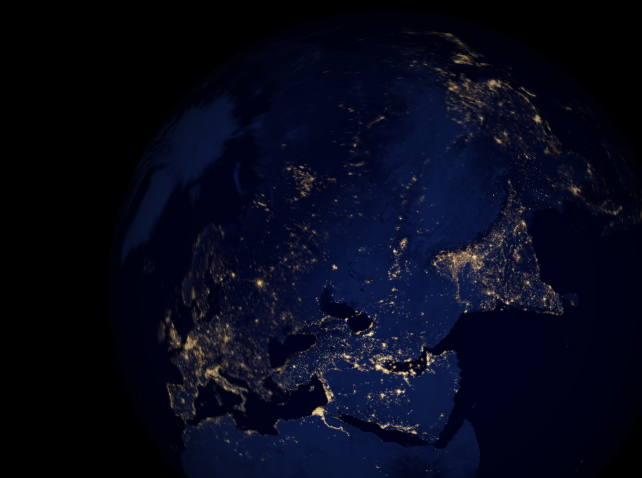
##################################################################
## Initial configuration
##################################################################
## Clone or download the repository and set the working directory
## with setwd to the folder where the repository is located.

Sys.setlocale("LC_TIME", 'C')

##################################################################
## Data
##################################################################

library(raster)
library(rasterVis)

cft <- brick('data/cft_20130417_0000.nc')
## set projection
projLCC2d <- "+proj=lcc +lon_0=-14.1 +lat_0=34.823 +lat_1=43 +lat_2=43 +x_0=536402.3 +y_0=-18558.61 +units=km +ellps=WGS84"
projection(cft) <- projLCC2d
##set time index
timeIndex <- seq(as.POSIXct('2013-04-17 01:00:00', tz = 'UTC'), length = 96, by = 'hour')
cft <- setZ(cft, timeIndex)
names(cft) <- format(timeIndex, 'D%d_H%H')

##################################################################
## Spatial context: administrative boundaries
##################################################################

library(maptools)
library(rgdal)
library(maps)
library(mapdata)

## Project the extent of the cft raster to longitude-latitude, because
## the map package works with it.
projLL <- CRS('+proj=longlat +datum=WGS84 +ellps=WGS84 +towgs84=0,0,0')
cftLL <- projectExtent(cft, projLL)
cftExt <- as.vector(bbox(cftLL))
## Extract the lines from the map package using this extent
boundaries <- map('worldHires',
                  xlim = cftExt[c(1, 3)], ylim = cftExt[c(2, 4)],
                  plot = FALSE)
## Convert the result to a SpatialLines object
boundaries <- map2SpatialLines(boundaries, proj4string = projLL)
## Project to the projection of the cft object
boundaries <- spTransform(boundaries, CRS(projLCC2d))

##################################################################
## Producing frames and movie
##################################################################

cloudTheme <- rasterTheme(region = brewer.pal(n = 9, 'Blues'))

tmp <- tempdir()
trellis.device(png, file = paste0(tmp, '/Rplot%02d.png'),
               res = 300, width = 1500, height = 1500)
levelplot(cft, layout = c(1, 1), par.settings = cloudTheme) +
    layer(sp.lines(boundaries, lwd = 0.6))
dev.off()

old <- setwd(tmp)
## Create a movie with ffmpeg ...
system2('ffmpeg',
        c('-r 6', ## with 6 frames per second
          '-i Rplot%02d.png', ## using the previous files
          '-b:v 300k', ## with a bitrate of 300kbs
          'output.mp4')
        )
file.remove(dir(pattern = 'Rplot'))
file.copy('output.mp4', paste0(old, '/figs/cft.mp4'), overwrite = TRUE)
setwd(old)

##################################################################
## Static image
##################################################################

levelplot(cft,
          layers = 25:48, ## Layers to display (second day)
          layout = c(6, 4), ## Layout of 6 columns and 4 rows
          par.settings = cloudTheme,
          names.attr = paste0(sprintf('%02d', 1:24), 'h'),
          panel = panel.levelplot.raster) +
    layer(sp.lines(boundaries, lwd = 0.6))

library(rgl)

clear3d()

pal <- colorRampPalette(brewer.pal(n = 9, 'Blues'))

N <- nlayers(cft)

ids <- lapply(seq_len(N),
              FUN = function(i)
                  plot3D(cft[[i]],
                         maxpixels = 1e3,
                         col = pal,
                         adjust = FALSE, ## Disable automatic scaling of xy axes.
                         zfac = 200)) ## Common z scale for all graphics

rglwidget() %>%
    playwidget(start = 0, stop = N,
               subsetControl(1, subsets = ids))

##################################################################
## Point space-time data
##################################################################

##################################################################
## Initial snapshot
##################################################################

library(gridSVG)
## Initial parameters
start <- NO2st[,1]
## values will be encoded as size of circles,
## so we need to scale them
startVals <- start$vals/5000

nStations <- nrow(airStations)
days <- index(NO2zoo)
nDays <- length(days)
## Duration in seconds of the animation
duration <- nDays*.3

library(grid)

## Auxiliary panel function to display circles
panel.circlesplot <- function(x, y, cex, col = 'gray',
                              name = 'stationsCircles', ...){
    grid.circle(x, y, r = cex,
                gp = gpar(fill = col, alpha = 0.5),
                default.units = 'native', name = name)
}

pStart <- spplot(start, panel = panel.circlesplot,
                 cex = startVals,
                 scales = list(draw = TRUE), auto.key = FALSE)
pStart

##################################################################
## Intermediate states to create the animation
##################################################################

## Color to distinguish between weekdays ('green') and weekend
## ('blue')
isWeekend <- function(x) {format(x, '%w') %in% c(0, 6)}
color <- ifelse(isWeekend(days), 'blue', 'green')
colorAnim <- animValue(rep(color, each = nStations),
                       id = rep(seq_len(nStations), nDays))

## Intermediate sizes of the circles
vals <- NO2st$vals/5000
vals[is.na(vals)] <- 0
radius <- animUnit(unit(vals, 'native'),
                   id = rep(seq_len(nStations), nDays))

## Animation of circles including sizes and colors
grid.animate('stationsCircles',
             duration = duration,
             r = radius,
             fill = colorAnim,
             rep = TRUE)

##################################################################
## Time reference: progress bar
##################################################################

## Progress bar
prettyDays <- pretty(days, 12)
## Width of the progress bar
pbWidth <- .95
## Background
grid.rect(.5, 0.01, width = pbWidth, height = .01,
          just = c('center', 'bottom'),
          name = 'bgbar', gp = gpar(fill = 'gray'))

## Width of the progress bar for each day
dayWidth <- pbWidth/nDays
ticks <- c(0, cumsum(as.numeric(diff(prettyDays)))*dayWidth) + .025
grid.segments(ticks, .01, ticks, .02)
grid.text(format(prettyDays, '%d-%b'),
          ticks, .03, gp = gpar(cex = .5))
## Initial display of the progress bar
grid.rect(.025, .01, width = 0,
          height = .01, just = c('left', 'bottom'),
          name = 'pbar', gp = gpar(fill = 'blue', alpha = '.3'))
## ...and its animation
grid.animate('pbar', duration = duration,
             width = seq(0, pbWidth, length = duration),
             rep = TRUE)
## Pause animations when mouse is over the progress bar
grid.garnish('bgbar',
             onmouseover = 'document.rootElement.pauseAnimations()',
             onmouseout = 'document.rootElement.unpauseAnimations()')

grid.export('figs/NO2pb.svg')

##################################################################
## Time reference: a time series plot
##################################################################

## Time series with average value of the set of stations
NO2mean <- zoo(rowMeans(NO2zoo, na.rm = TRUE), index(NO2zoo))
## Time series plot with position highlighted
pTimeSeries <- xyplot(NO2mean, xlab = '', identifier = 'timePlot') +
    layer({
        grid.points(0, .5, size = unit(.5, 'char'),
                    default.units = 'npc',
                    gp = gpar(fill = 'gray'),
                    name = 'locator')
        grid.segments(0, 0, 0, 1, name = 'vLine')
    })

print(pStart, position = c(0, .2, 1, 1), more = TRUE)
print(pTimeSeries, position = c(.1, 0, .9, .25))

grid.animate('locator',
             x = unit(as.numeric(index(NO2zoo)), 'native'),
             y = unit(as.numeric(NO2mean), 'native'),
             duration = duration, rep = TRUE)

xLine <- unit(index(NO2zoo), 'native')

grid.animate('vLine',
             x0 = xLine, x1 = xLine,
             duration = duration, rep = TRUE)

grid.animate('stationsCircles',
             duration = duration,
             r = radius,
             fill = colorAnim,
             rep = TRUE)

## Pause animations when mouse is over the time series plot
grid.garnish('timePlot', grep = TRUE,
             onmouseover = 'document.rootElement.pauseAnimations()',
             onmouseout = 'document.rootElement.unpauseAnimations()')

grid.export('figs/vLine.svg')

library(rgl)
library(magick) ## needed to import the texture

## Opens the OpenGL device with a black background
open3d()
bg3d('black')

## XYZ coordinates of a sphere
lat <- seq(-90, 90, len = 100) * pi/180
long <- seq(-180, 180, len = 100) * pi/180
r <- 6378.1 # radius of Earth in km
x <- outer(long, lat, FUN = function(x, y) r * cos(y) * cos(x))
y <- outer(long, lat, FUN = function(x, y) r * cos(y) * sin(x))
z <- outer(long, lat, FUN = function(x, y) r * sin(y))

## Read, scale, and convert the image
nightLightsJPG <- image_read("https://eoimages.gsfc.nasa.gov/images/imagerecords/79000/79765/dnb_land_ocean_ice.2012.13500x6750.jpg")
nightLightsJPG <- image_scale(nightLightsJPG, "8192") ## surface3d reads files up to 8192x8192
nightLights <- image_write(nightLightsJPG, tempfile(),
                           format = 'png') ## Only the png format is supported
## Display the sphere with the image superimposed
surface3d(-x, -z, y,
          texture = nightLights,
          specular = "black", col = 'white')

writeWebGL('nightLights', width = 1000)

cities <- rbind(c('Madrid', 'Spain'),
                c('Tokyo', 'Japan'),
                c('Sidney', 'Australia'),
                c('Sao Paulo', 'Brazil'),
                c('New York', 'USA'))
cities <- as.data.frame(cities)
names(cities) <- c("city", "country")

library(XML)

geocode <- function(x){
    city <- x[1]
    country <- x[2]
    urlOSM <- paste0('http://nominatim.openstreetmap.org/search?',
                     'city=', city,
                     '&country=', country,
                     '&format=xml')
    ## Parse the webpage
    xmlOSM <- xmlParse(urlOSM)
    ## Use only the first result
    cityOSM <- getNodeSet(xmlOSM, '//place')[[1]]
    ## Extract attributes: longitude...
    lon <- xmlGetAttr(cityOSM, 'lon')
    ## and latitude
    lat <- xmlGetAttr(cityOSM, 'lat')
    ## Return them as a vector
    as.numeric(c(lon, lat))
}

points <- apply(cities, 1, geocode)
points <- t(points)
colnames(points) <- c("lon", "lat")

cities <- cbind(cities, points)

library(geosphere)

## When arriving or departing include a progressive zoom with 100
## frames
zoomIn <- seq(.3, .1, length = 100)
zoomOut <- seq(.1, .3, length = 100)

## First point of the route
route <- data.frame(lon = cities[1, "lon"],
                    lat = points[1, "lat"],
                    zoom = zoomIn,
                    name = cities[1, "city"],
                    action = 'arrive')

## This loop visits each location included in the 'points' set
## generating the route.
for (i in 1:(nrow(cities) - 1)) {

    p1 <- cities[i,]
    p2 <- cities[i + 1,]
    ## Initial location
    departure <- data.frame(lon = p1$lon,
                            lat = p1$lat,
                            zoom = zoomOut,
                            name = p1$city,
                            action = 'depart')

    ## Travel between two points: Compute 100 points between the
    ## initial and the final locations.
    routePart <- gcIntermediate(p1[, c("lon", "lat")],
                                p2[, c("lon", "lat")],
                                n = 100)
    routePart <- data.frame(routePart)
    routePart$zoom <- 0.3
    routePart$name <- ''
    routePart$action <- 'travel'

    ## Final location
    arrival <- data.frame(lon = p2$lon,
                          lat = p2$lat,
                          zoom = zoomIn,
                          name = p2$city,
                          action = 'arrive')
    ## Complete route: initial, intermediate, and final locations.
    routePart <- rbind(departure, routePart, arrival)
    route <- rbind(route, routePart)
}

## Close the travel
route <- rbind(route,
               data.frame(lon = cities[i + 1, "lon"],
                          lat = cities[i + 1, "lat"],
                          zoom = zoomOut,
                          name = cities[i+1, "city"],
                          action = 'depart'))

summary(route)

## Function to move the viewpoint in the RGL scene according to the
## information included in the route (position and zoom).
travel <- function(tt){
  point <- route[tt,]
  rgl.viewpoint(theta = -90 + point$lon,
                phi = point$lat,
                zoom = point$zoom)
}

## Examples of usage of travel
## First frame
travel(1)
rgl.snapshot('images/travel1.png')
## Frame no.1200
travel(1200)
rgl.snapshot('images/travel2.png')

movie3d(travel,
        duration = nrow(route),
        startTime = 1, fps = 1,
        type = 'mp4', clean = FALSE)